Continuous Level Transform1
Introduction
Be reminded that units serving as the second, passive component of a Driver/Transform coupling
have a primary purpose which is fully reliable and a secondary purpose which is less so. The primary purpose
of a Transform is to adapt the values of a
driver-domain sequence to a specified range. The secondary purpose
is to obtain a distribution across that range, concentrating
values in some regions and dispersing them away from others. The transform achieves this secondary purpose using
quantile functions, which are effective only to the extent that the source
sequence is uniform.
Of the Driver units surveyed on this site, only
Balance produces reliably uniform sequences
over the short term.
DriverSequence also produces short-term uniformity,
but only if (1) the source samples are themselves uniform and (2) the sequence length is a multiple of the source-sample count.
The standard random-number generator (implemented as Lehmer)
only tends toward uniformity with large enough sequence lengths to permit the
law of large numbers to exert influence.
Borel and
Moderate also tend towards uniformity, but even
longer sequence lengths are required to make this reliable. Brownian
is decidedly non-uniform over the short term, while the chaotic drivers Logistic
and Baker are not uniform on any scale.
Suppose then that you like the shape or the pattern produced by one of these non-uniform drivers but you also want the
overall content of a transformed sequence to conform to a particular distribution. Is there a way to level (flatten out) the
driver sequence while retaining the relative ups and downs of sample values? To do this would require dividing the
driver domain into intervals, then resizing those intervals relative to one another. Overpopulated intervals would expand,
while underpopulated intervals would contract — and unpopulated intervals would be minimized. This, in a
nutshell, is how the ContinuousLevel transform works.
Since ContinuousLevel maps the driver domain back onto itself, it can serve as a
decorator interposing between a driver and
a second transform. In fact, that's actually the point, since ContinuousLevel
if used properly will give the second transform a uniformly distributed source, which the second transform can now reliably conform to the distribution
requested.
Usage
The actual mechanics of inferring the distribution of a non-uniform sequence, and then for countering it, will be explained shortly.
Before that we explore two scenarios illustrating how ContinuousLevel might be
used.
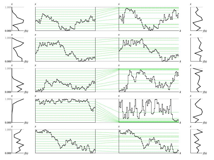
Scenario #1 (Figure 1 (a)) draws five sources from the Brownian
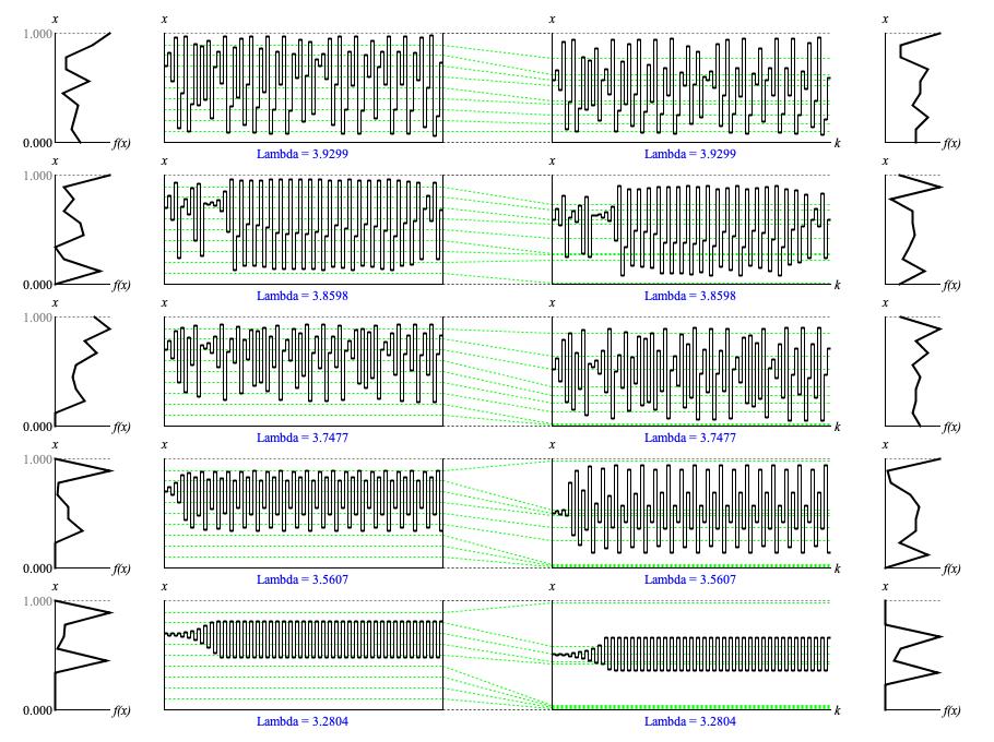
driver while scenario #2 (Figure 1 (b)) draws five sources from
Logistic.
All ten sequences were 75 samples in length, which was the largest number that would still fit before-and-after information into one horizontal row of graphs.

Figure 1 (a): Panel illustrating how
ContinuousLevel transforms five different
Brownian sequences. Each row of graphs provides a histogram
of the unleveled sequence (far left), a time-series graph of unleveled samples (middle left), a line diagram showing how
equal-sized intervals of the unleveled domain map to expanded or contracted intervals of the leveled domain (center), a time-series graph of
leveled samples (middle right), and a histogram of the leveled sequence (far right).
For scenario #1, the difference between shapes was due entirely to different random seeds.
The deviation control parameter σ was fixed at 0.0625 and the mode was
fixed at ContainmentMode.REFLECT.
Each Brownian source sequence was captured into a separate
Double array.
A separate ContinuousLevel instance was allocated for each captured
sequence. Property ContinuousLevel.itemCount
was set 10, dividing the driver domain into the ten equal-height bands shown in the unleveled sample graphs in the middle left of Figure 1 (a).
This averaged 75/10=7.5 samples per histogram interval. Method ContinuousLevel.analyze()
was used to adapt each separate ContinuousLevel instance to its associated source
sequence. The source sequence was then processed through ContinuousLevel to produce
the leveled sample graphs in the middle right of Figure 1 (a).
The effectivenesss of each leveling process can best be assessed by comparing the before histogram on the far left with the after
histogram on the far right. These histogram graphs divided the range into 10 regions, and connected the resulting tallies with line
segments. That the after histograms still have substantial troughs reflects both the short sequence length and the
coarse setting of ContinuousLevel.itemCount=10.
However the before histrograms have even more dramatic troughs, often dropping entirely down to zero over a stretch, and these features are
generally mitigated in the after histograms.

Figure 1 (b): Panel illustrating how
ContinuousLevel transforms five different
Logistic sequences. Each row of graphs provides a histogram
of the unleveled sequence (far left), a time-series graph of unleveled samples (middle left), a line diagram showing how
equal-sized intervals of the unleveled domain map to expanded or contracted intervals of the leveled domain (center), a time-series graph of
leveled samples (middle right), and a histogram of the leveled sequence (far right).
For scenario #2, the difference between shapes comes from different lambda
values, starting up near the parameter maximum of 4 and decreasing toward the parameter minimum of 3. The starting value for
each sequence is fixed at 0.7 (selected by eyeballing the lowermost sequence), while the random seed is irrelevant since
Logistic makes no use of the random number generator.
As in Scenario #1, each Logistic source sequence was captured into a separate
Double array and a separate ContinuousLevel
instance was adapted to the corresponding sequence.
Recall that logistic sequences undergo a bifurcation process, with initially just one attractor (point of concentration), then 2 (e.g. for λ=3.2804), then more until the attractors become a smear and the smear ultimately covers the entire range from zero to unity. Little benefit is gained by leveling the λ=3.2804 sequence, but already with λ=3.2804 what looks like variation around one attractor in the second-from-top interval (unleveled from 0.8 to 0.9) expands out to three clearly distinct attractors after leveling. But look also the row of graphs for λ=3.8598. In the topmost interval what looks like iterated values expands into a descending contour, while in the bottommost interval another set of iterations expands to reveal a clear upward trend.
Originally when I prepared this graphic I made the assumption that the distribution of values in the topmost sequence is something
that the other sequences trend toward. This led me to allocate just one ContinuousLevel
instance, to adapt it only to the topmost sequence, but to apply it to all five sequences.
All five rows in the original panel exhibited the same mapping of equal-sized intervals in the before sample graph to
expanded/contracted intervals in the after sample graph.
This is a reasonable approach to take when you're generating a Logistic while
varying lambda continuously over time. However when lambda
is static, the most benefit is gained by leveling separately.
Coding
ContinuousLevel implementation class.
The type hierarchy for ContinuousLevel is:
-
TransformBase<T extends Number> extends WriteableEntity implements Transform<T> -
ContinuousDistributionTransform extends TransformBase<Double> implements Transform.Continuous -
ContinuousLevel
                  extends ContinuousDistributionTransform
                  implements Driver
The ContinuousLevel transform satisfies the Transform
interface, in that it draws input from the driver domain; however it turns right around and maps
its output right back into the same domain. As such, the ContinuousLevel transform also satisfies the
Driver interface. It would therefore reason in a preparatory phase to capture a
non-uniform set of driver values in a DriverSequence and use
the captured content to adapt a ContinuousLevel instance. A second, generative phase would pipe output from
the DriverSequence through the same ContinuousLevel instance and
additionally through a DiscreteWeighted. The resulting now-reliably weighted
indices could be used to select, say, a pitch from a scale.
Through its ContinuousDistributionTransform superclass,
ContinuousLevel transform leverages an embedded
ContinuousDistribution instance.
A ContinuousDistribution is itself a composite of
ContinuousDistributionItem instances, each instance being described
by four fields:
-
The
leftandrightfields specify which segment of the distribution range the item covers. -
The
originfield specifies the relative density of range values aroundleft. -
The
goalfield specifies the relative density of range values aroundright.
The actual work of converting driver values into range values is shouldered by
ContinuousDistribution.quantile().
This method determines which ContinuousDistributionItem applies by dividing the driver
domain into irregular intervals, one for each ContinuousDistributionItem. Whichever
interval the driver value falls into, the corresponding ContinuousDistributionItem
becomes responsible for placing the transformed value in that particular portion of the distribution range.
The width of the portion is determined by the relative area under the probability density curve
for the corresponding ContinuousDistributionItem.
This area is given by range (portion width) times average probability or:
(right-left)×(origin+goal)/2
All that has just been described is taken care of by ContinuousDistributionTransform,
but the mechanisms for creating the ContinuousDistributionItem instances are peculiar to
ContinuousLevel and specifically to the
deriveDistribution() method.
Preparatory to using deriveDistribution(), the captured sequence of driver values must be analyzed by a
ContinuousHistogram
instance. The histogram divides the driver domain into equal-sized intervals and counts the number of sequence values falling in each interval.
Method ContinuousLevel.deriveDistribution()
uses the ContinuousHistogram analysis to derive
ContinuousDistributionItem instances which
expand densely populated histogram intervals and which compress sparsely populated intervals.
In what follows, let L be the number of histogram intervals. Let N be the total number of samples counted, let nk be the number of samples counted in the kth histogram interval, and let J be the number of histogram intervals for which nk=0.
As Figure 1 (a) and Figure 1 (a)
indicate, each of the L equal-sized histogram intervals will carry over to a separate ContinuousDistributionItem instance.
When a histgram interval has any content at all (nk>0), the portion of the output range associated with
the ContinuousDistributionItem can be sized by making:
(right-left) = nk/(N+J)
When a histgram interval is empty of content (nk=0), the range portion should be minimized:
(right-left) = 1/(N+J)
We cannot simply set right=left.
The fact that the histogram regions are equal sized means that every
ContinuousDistributionItem must have the same area under the probability density curve (see
above). But if the range of a ContinuousDistributionItem falls to zero, then the
area under the curve must also fall to zero.
The adjustment to the denominator is necessary because the minimal (single-sample) amounts used to calculate ContinuousDistributionItem
widths are not reflected in the total sample count N.
Assigning each ContinuousDistributionItem
an equal share of the probability domain means setting:
(right-left)×(origin+goal)/2 = 1/L
Since the histogram analysis provided only the count of samples over an entire interval, not the relative densities at the left and right
extremes, we stipulate that the origin and goal
can be populated using the same local variable weight:
(right-left)×weight = 1/L
Solving for weight gives:
weight = N×(right-left) = L×(N+J)/nk
analyze() has three flavors — that is, argument signatures. The flavor used to
process the Brownian and Logistic sequence graphed above was analyze(Double[]).
If collections are preferred to arrays, an alternative is
analyze(List<Double>).
If the source sequence has been captured within a DriverSequence instance, there's analyze(DriverSequence sequence).
Comments
- The present text is adapted from my Leonardo Music Journal article from 1993, "How To Level a Driver Sequence".
- The meaning of the "area under the curve" with respect to probability density functions is explained in this site's "basics" presentation on statistical distributions.
| © Charles Ames | Page created: 2022-08-29 | Last updated: 2022-08-29 |