Standard Randomness: Lehmer¹

Introduction

The Lehmer driver produces sequences which are independent over the short term and uniform over the long term. It does so by wrapping Java's standard random number generator, java.util.Random, whose characteristics with regard to independence and uniformity are demonstrated elsewhere on this site.

The Lehmer driver establishes the baselines against which all other Driver implementations may be evaluated. Its

The Lehmer driver bears a particular relation to Balance, the balanced-bit driver. Output from both these drivers nominally follows a continuous uniform distribution; however, only Lehmer realizes this distribution over the short term. In that sense Lehmer is the continuous counterpart of the urn model's selection with replacement, just as Balance is the continuous counterpart of selection without replacement.

Profile

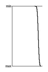
Figure 1 illustrates Lehmer output with a sequence of 200 samples generated with a random seed of 1.

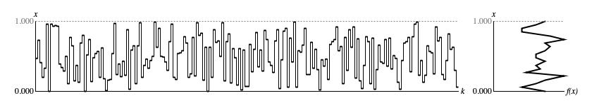
Figure 1: Sample output from Lehmer.next(). The left graph displays samples in time-series while the right graph presents a histogram analyzed from the same samples.

The vertical x axes for both graphs represent the driver domain from zero to unity; the horizontal k axis of the time-series graph (left) plots ordinal sequence numbers; the horizontal f(x) axis of the histogram (right) plots the relative concentration of samples at each point in the driver domain.

Bitwise Analysis

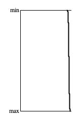
Figure 2 takes the sequence shown in Figure 1 and breaks out what happens in bit 1 (zero or one-half), bit 2 (zero or one-quarter), bit 3 (zero or one-eighth), bit 4 (zero or one-sixteenth), and the residual bits (continuous between zero and one-sixteenth).

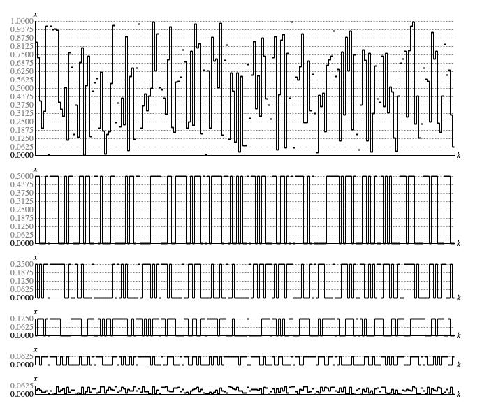
Figure 2: Bitwise analysis of a sequence generated by Lehmer.next().

I have demonstrated the independence previously of sequences produced by java.util.Random.nextBoolean(), which presumably operates by extracting the most significant bit from a linear-congruence value. Since the independence of the four most significant bits was also demonstrated, it stands to reason that each of bits 2-4 should also be independent.

The bit-specific graphs in Figure 2 transition back and forth between a set state (bit value 1) and a clear state (bit value 0). If the probability of transitioning is truly 1 in 2, then the number of samples between transitions should follow a geometric distribution with "probability of success" 0.5. This distribution predicts transition-to-transition sample counts will happen in the proportions given in the top row of Table 1. The remaining rows of Table 1 provide the actual stats for these bit-specific graphs. Although specific actual percentages differ substantially from the predictions, the downward trends are mostly consistent. The one oddity is that the "5 or more" percentage always exceeds the "4 Samples" percentage; yet these "5 or more" results are not out of line with the predicted 6.25%.

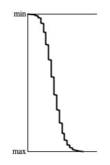
Figure 3: Histogram of sample-to-sample differences from Lehmer.next() after 10,000 consecutive samples.

Transitions

The sample-to-sample difference Δx_k is calculated as x_k − x_k-1. Figure 3 plots the range of sample-to-sample differences along the vertical Δx axis against the relative concentrations of these values along the horizontal f(Δx) axis. Remember that sample values are limited to the range from zero to unity. The largest downward leap can be from the top of the range (x_k-1 = 1.0) to the bottom (x_k = 0.0) giving 0.0 − 1.0 = -1.0. The largest upward leap can be from the bottom of the range (x_k-1 = 0.0) to the top (x_k = 1.0) giving 1.0 − 0.0 = 1.0. The histogram in Figure 3 divided this range into 40 intervals, 20 below zero and 20 above. 10,000 calls to Lehmer.next() were required until the histogram smoothed out enough to determine a trend. The inferred distribution rises linearly from 0 for the full downward leap to a maximum for small movements and then falls back linearly to 0 for the full upward leap.

The standard deviation of Δx around zero is 0.410, which provides a baseline against which other drivers can be evaluated. This summary statistic embraces both upward and downward transitions but is equally valid for upward transitions, specifically, and downward transactions, specifically. Lower standard deviations suggest a proximity dependence, which grows stronger as the deviation reduces toward zero. Higher deviations indicate a proximity aversion.

Independence

I demonstrated the independence of 4-nibble sequences from java.util.Random.nextDouble() by using summary statistics to show that the tallies of 4-nibble patterns converged, over the long term, toward their average. These statistics were presented as Table 2 on the page Basics I: Randomness. It would be redundant to repeat those statistics here; however it occured to me that the point could be made more intuitively if I could graph the trend from short to long. Even though such a graphic would provide no insight into what kinds of patterns were favored or disfavored, this would at least provide a mechanism for reducing 16×16×16×16 = 65,536 tallies to a readily comprehensible picture.

Figure 4(a): Divergence of 4-nibble pattern counts from Lehmer.next() with 10 samples per pattern.

Figure 4(b): Divergence of 4-nibble pattern counts from Lehmer.next() with 100 samples per pattern.

Figure 4(c): Divergence of 4-nibble pattern counts from Lehmer.next() with 1,000 samples per pattern.

Figure 4(d): Divergence of 4-nibble pattern counts from Lehmer.next() with 10,000 samples per pattern.

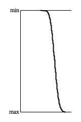
Figures 4(a), 4(b), 4(c), and 4(d) each reduce 65,536 4-nibble pattern tallies to trend graphs. The graphs are all 100 pixels high. They were derived by sorting the tallies into ascending order and by stepping through at a rate of 65,536/100 = 655 tallies per pixel. For the population sizes, one "sample" means a 4-nibble sequence. Thus where Figure 4(a) says "10 samples per pattern", that means 10×65,536×4 = 2,621,440 calls to Lehmer.next(). Each subsequent graph multiplies the number of calls by 10. The four graphs presented here correspond to the four bottom rows of summary statistics presented in Table 2.

Inspecting these graphs visually, the progress of convergence around the average tally value is clear. However it required 1,000 samples per pattern to suggest convergence and a full 10,000 samples per pattern to assert that convergence is happening. That's a whopping 2,621,440,000 calls to Lehmer.next() (and commensurate with the cycle length of java.util.Random!). This establishes a baseline; all remaining Driver implementations are dependent in some manner, so when applying this 4-nibble independence test to other drivers, rising trends should be consistent.

/**
 * Instances of the {@link Lehmer} class generate a driver sequence
 * using Java's built in random generator.
 * All {@link Lehmer} instances delegate selection to the
 * {@link SharedRandomGenerator} singleton.  This in turn wraps a
 * single instance of {@link java.util.Random}.
 * @author Charles Ames
 */
public class Lehmer extends DriverBase {
   /**
    * Constructor for {@link Lehmer} instances with container.
    * @param container An entity which contains this driver.
    */
   public Lehmer(WriteableEntity container) {
      super(container);
   }
   /**
    * Constructor for {@link Lehmer} instances without container.
    */
   public Lehmer() {
      this(null);
   }
   @Override
   protected double generate() {
      return random.nextDouble();
   }
}

Coding

The type hierarchy for Lehmer is:

• DriverBase extends WriteableEntity implements Driver
• Lehmer extends DriverBase

Listing 1 provides the source code for the Lehmer class. All this class really does is repackage java.util.Random in a wrapper that satisfies the Driver interface. The constructor acquires the shared instance of java.util.Random from the SharedRandomGenerator singleton and stores this instance locally. The java.util.Random.nextDouble() call is made by Lehmer.generate(), which is not public facing. Instead, generate() is called by DriverBase.next(), which takes care that the previous sequence value is properly managed.

Comments

1. The present text is adapted from my Leonardo Music Journal article from 1992, "A Catalog of Sequence Generators". The heading is "Lehmer's 'Linear Congruence' Formula", p. 58.