Design I: Driver/Transform

Introduction

In the driver/transform design, an active Driver generates an intermediate value u in the continuous "driver domain" from zero to unity, while a passive Transform distributes u values over whatever "target range" a particular application requires. This target range can be either discrete (values are integers) or continuous (values are real — floating point — numbers).

Thus arose the paradigm of a system coupling an active “driver” with a passive “transform”. My usage of “driver” came from acoustics, where a “driver” indicates an active component (e.g. the vocal cords) that would be coupled with a passive resonating system (e.g. the cavities of the mouth and nose). The range from zero to unity became known as the “driver range”.

Intermediate driver values are ideally dispersed uniformly over the driver domain. "Uniformly" means that if you divide the domain into equal-sized regions, the counts of values falling into these regions will, over the long term, come into agreement. While the specific domain extent from zero to unity is mandatory, the ideal of uniformity is optional.
If the target range is discrete, the transform divides the driver domain into consecutive regions, each associated with target value. The wider the region, the higher relative count of values in sequences over the long term.
If the target range is continuous, the transform builds what's called a cumulative distribution function F, where F(X) indicates the long-term proportion of sequence elements with values x ≤ X. Now given a target range from A to B, the cumulative distribution function is an always rising curve with F(A) = 0 and F(B) = 1. And because the curve is always rising it is always invertible, which means that given a driver value u there will always be exactly one corresponding x value such that u = F(x).

If one can generate a driver sequence whose values X₀, X₁, X₂, …, X_N-1 are uniformly distributed in the continuous domain from zero to unity (and the conventional random-number generator is an example of this), then one can conform this sequence to any desired distribution by applying an appropriate statistical transform. How to do this will be explained later. Hence we gain modularity and flexibility without losing generality if the Driver contract stipulates that continuous sequences be 'normalized' to range from zero to unity. Readers should bear in mind that non-uniformity in the driver sequence will persist through the transformation into the final result. The overall target range will be valid, but local concentrations inside that range may stray from the distribution. Since it is difficult to estimate in advance how nonuniform drivers will affect a transform, it is often helpful to graph an empirical histogram of driver/transform output so one can evaluate the resulting distribution visually.

The Driver Domain

Within the Driver/Transform design, the Transform.convert() method acts as a mathematical function mapping values from a source set, the domain, to a target set, which in my day was called the range. I have adopted the term driver domain for the source set, since this set describes values produced specifically by Random.nextDouble() and more generally by Driver.next(). The driver domain is synonymous with the probability domain associated with statistical distributions, though the contexts differ.

Mathematically, driver domain values are real numbers. Real numbers are "continuous" in the sense that given any two numbers which are different (but possibly very close), the number half-way between is also a real number. This means that real numbers can be represented — up to a certain precision — in binary form with digits to the right of the binary point. Real numbers are thus distinguished from integers which are discrete and which have no digits right of the binary point. Real numbers are implemented on this site using Java's double type; other representations are available (e.g. float), but double is what most hardware floating-point processing units work with.

The driver domain runs from zero to unity. But for unity, driver values all have zero to the left of the binary point.

Adapting to a Range

Experience gained from Random.nextDouble() shows this: Having the driver domain extend continuously from zero to unity greatly simplifies the calculations needed to convert to other ranges. For example mapping the driver value u into the continuous range from A to B uses the calculation:

(B-A)*u + A.

Likewise, mapping the driver value u into the discrete range from 0 (inclusive) to N (exclusive) uses the calculation:

Math.floor(N*u).

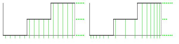
Figure 1: Graph of probability density function for the continuous uniform distribution ranging from zero to one.

Conforming to a Distribution

Figure 1 illustrates why uniform driver values are desirable when the distribution matters. Two graphs are presented. Each x-axis plots the driver range from zero to unity. Each y-axis plots the discrete target range {0, 1, 2}. The transformation from driver to target output is accomplished by step functions, which in each graph map 1/3 of the driver range to outcome 0, 1/3 of the driver range to outcome 1, and 1/3 of the driver range to outcome 2. The vertical green lines represent specific driver values, while the rows of green dots tally how many verticals intersect with the step function at that particular output.

Notice that the driver values on the left graph are spaced in equal horizontal increments. Values are no more concentrated in the middle of the driver range than they are at either end. In other words, the driver values for the left graph are unform. Verticals intersect the step function in five places at each target value. Thus the statistical distribution of target values accurately reflects the distribution that the step function was designed to produce.
Notice that the driver values on the right graph are more concentrated at either end of the driver range than they are in the middle. Here the driver values are non-unform. Verticals intersect the step function in six places for target values 0 and 2, but in only three places for target value 1. Therefore the statistical distribution of target values in the right graph does not accurately reflect the distribution that the step function was designed to produce.

Leveling Driver Values

A statistical transform is reliable only to the extent that its driving input is uniform. Yet among the implementators of Driver.next():

Only Balance distributes output values uniformly over the short term.
Lehmer (the standard random number generator) tends toward uniformity as the population size grows large enough for the Law of Large Numbers to exert influence.
DriverSequence will produce uniform sequences under two conditions: (1) the population of source samples is itself uniformly distributed, and (2) the sequence length is an integer multiple of the source population size.

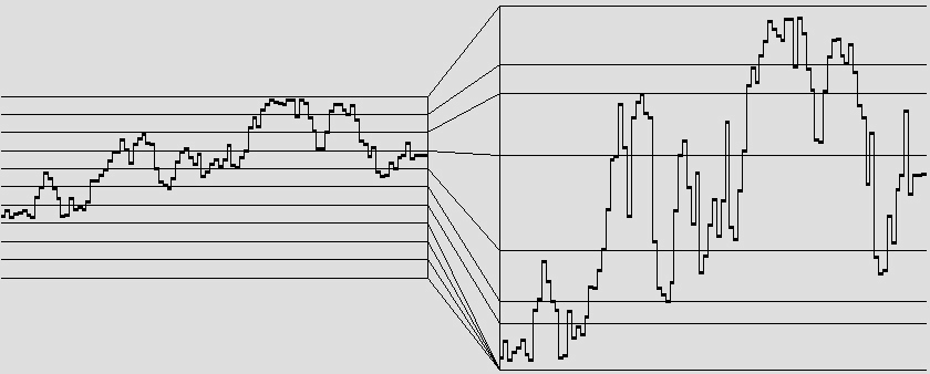
Figure 2: An unleveled Brownian sequence (left) and the same
sequence processed using the ContinuousLevel transform (right).

Most other implementations of Driver do not strive in any way for uniformity. For example, the sequence on the left side of Figure 2 was generated using the Brownian driver. None of these sequence values fall in the range from 0.0 to 0.3. The most dense region is that between 0.6 and 0.7; that's where the sequence lingered most during this particular run.

Referring back to Figure 1, if you are employing a transform for the purpose of adapting driver-domain values to the needs of a particular application, it may not be of great concern to you that range values 0 and 2 are over-represented by comparison to range value 1. However if conformance to the distribution is essential to what you are trying to achieve, then you need some way of performing the operation shown in Figure 2, which retains the up-and-down contour of the original Brownian sequence, but which compresses sparsely populated regions (reducing empty regions down to nothing) and expands densely population regions so that equal-sized intervals afterward contain roughly the same number of samples.

The ContinuousLevel unit performs the operation illustrated in Figure 2. Although built upon the Transform base class, ContinuousLevel also implements the Driver interface. Thus ContinuousLevel maps driver-domain values right back into the driver domain, adapting non-uniform output from a 'real' Driver into uniform input for another Transform.

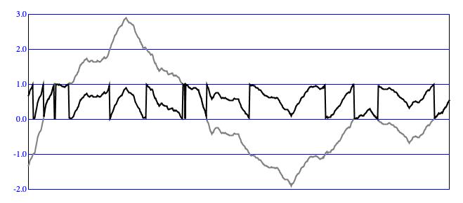
Figure 3: An uncontained Brownian sequence (gray), and
the same sequence processed using the WRAP ContainmentMode.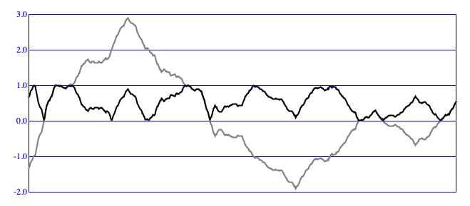

Figure 4: An uncontained Brownian sequence (gray), and
the same sequence processed using the REFLECT ContainmentMode.

Containing Within the Domain

The majority of processes implementing the Driver operate between well-defined lower and upper bounds which are thus readily scalable to the driver domain from zero to unity. In principle one should be able to exploit any desired sequence, regardless of origin. The capability to accept fully fleshed-out value sequences and to rescale these to the driver domain is particular to the One exception is DriverSequence, which presents values sequentially from a stored array which must be populated prior to the first call to DriverSequence.next(). However since the entire source set is known in advance, it is straightforward enough to ascertain lower and upper bounds, then use these bounds to rescale the set.

Two other exceptions are Brownian and Bolt, both of which are based upon Brownian motion. Brownian motion starts with some arbitrary location, and with each iteration moves randomly from wherever it was to wherever it will be.¹ The identical gray contours in Figure 3 and Figure 4 exemplify Brownian motion, plotting locations along the y-axis and time (actually sequential order) along the x-axis.

Comments

Historically what Brown observed in his new-fangled microscope was two-dimensional. The one-dimensional nature of Driver.next{} accomodates either the left-right (x) or the up-down (y) component, but a pair of generators will produce two-dimentional motion if desired.

Page created: 2022-08-29

Last updated: 2022-08-29