Basics I: Randomness1
Overview
This page's first topic, Java's Random Class, explains how
Java's built-in java.util.Random generator uses a deterministic algorithm to generate
sequences of numbers which behave as if they were random.
The second topic, Verifying Random Behavior focuses on two behaviors which we would expect from random sequences:
- uniformity over the long term and
- independence over the short term.
The topic
both explains what these behaviors mean and verifies that sequences from java.util.Random
behave as described. It also discusses how the Law of Large Numbers reconciles
the short term to the long term.
The third topic, Seeding the Random Generator, offers practical advice on seeding the random generator; also on how the approach to seeding relates to how sequences will be used.
The fourth topic, Sharing the Random Generator discusses parallel sequence-streams
and whether it is desirable to instantiate separate java.util.Random
instances for each stream (with independent seeds) or to share a single instance of java.util.Random
between all streams.
The fifth topic, Random Shuffling explains what shuffles are good for, and how they work.
The closing topic of this page, Singleton Coding provides a listing of my
SharedRandomGenerator class, which wraps java.util.Random.
Java's Random Class
Java's standard random number generator java.util.Random employs the
linear congruence formula first described in 1949 by Derrick Henry
Lehmer. The formula uses unsigned modular arithmetic
based on a modulus M, where any integer value outside the range from 0 to
M-1 is wrapped back into that range. Here is the linear congruence formula:
Of the symbols, A is a constant multiplier, B is a constant increment, and M is the constant modulus. Each iteration of this formula operates upon the result of the previous iteration Xk-1. The initial value X0 is called the seed of the random sequence. Starting with a particular seed will generate the same sequence every time.
- The "linear" step of the formula calculates AXk-1+B. The formula works best when the product AXk-1 is, more often than not, substantially greater than M
- The "congruence" step of the formula wraps the "linear" result back into the range from 0 to M-1. This "congruence" step is similar to taking a decimal fraction such as 0.679570457114761 discarding the four leftmost digits to obtain 0.70457114761.
According to Oracle's Java Platform Documentation for the
Random class,
Lehmer's linear congruence formula is implemented within Java's protected
Random.next()
method. You can't access this fundamental method directly. Rather, other methods request a raw bit pattern from Random.next(),
then convert this raw result to numeric datatype such as int,
double, or even boolean.
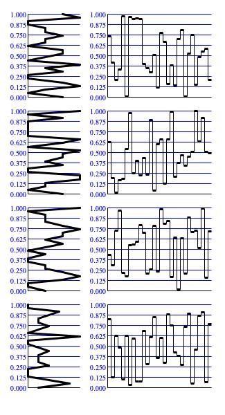
Figure 1: Example 32-element sequences generated by
Random.nextDouble() with different
random seeds.
The Random.next() method implements the linear congruence formula with A = 0x5DEECE66DL = 25,214,903,917,
B = 0xBL = 11,
and M = 248 = 281,474,976,710,656.
Calculations are undertaken using an unsigned long (64-bit) integer so, since M is the 48th power of two, the act of applying
the modulus is effected simply by masking out the 16 most significant bits. The documentation also suggests that
only 32 of the remaining 48 bits exhibit sufficently 'random' behavior, so Random.next() presents at most
bits 17 to 48 of the long word to its calling method.
For the record, M/A = 11,163 and 11,163/M = 0.00000000004. This means that the product AXk-1 will be substantially larger than M for all but a miniscule number of values of Xk-1. Thus the step of discarding the most-significant bits will happen during nearly every iteration of Java's linear congruence implementation.
Also for the record, there are competing schools of thought about how M, A, and B should be chosen. The Wikipedia entry on the linear congruential generator lists parameters for 21 different implementations of Lehmer's formula and comments on strengths and weaknesses of various choices. Java's particular implementation is not singled out for criticism, which is reassuring to me given Java's status on the present site.
The methods which convert raw bit patterns from Random.next() into usable numeric formats include the following:
-
Random.nextBoolean()produces eithertrueorfalse; alternatively, heads or tails. -
Random.nextInt()produces 32-bit signed integers ranging from-232 = -2,147,483,648to232-1 = 2,147,483,647. -
Random.nextInt(int n)produces 32-bit signed integers in the range from0ton-1. -
Random.nextLong()produces 64-bit signed integers ranging from-264 = -9,223,372,036,854,775,808to264-1 = 9,223,372,036,854,775,807. -
Random.nextFloat()produces 32-bit (single precision) floating-point numbers ranging from zero to unity with 6-7 significant decimal digits. It achieves this by taking the quotientRandom.nextInt(232)/232. -
Random.nextDouble()produces 64-bit (double precision) floating-point numbers ranging from zero to unity. It likewise achieves this by taking the quotientRandom.nextInt(232)/232. Although the data type is capable of 15 significant decimal digits, the quantity 232 = 2,147,483,648 crops this number down to 9-10 digits.
Figure 1 presents four 32-element sequences generated using Random.nextDouble().
The histogram provided for each sequence is derived by partitioning the range from zero to unity into 24 equal regions, by counting the number of samples in each region, and by joining the
resulting tallies with line segments.
Verifying Random Behavior
People sometimes stress the point that numbers generated using the linear congruence formula are "pseudo" random, since an application which starts with a given seed will always generate the same sequence of values. To be truly random — according to this viewpoint — the numbers would need to come into the computer from a "natural" (non-digital) source. For example, Lejaren Hiller once told me that in early days random values were obtained by "sampling the voltage off a dirty transistor".
The question comes down to whether "pseudo" randomness suits the purposes it is being used for. If the purpose is submitting questions to divine intervention through an agency of chance (e.g. gambling), then a deterministic algorithm is probably not appropriate. If the purpose is to generate a new map for each session of a game, then "pseudo" randomness may be okay if the seed value is different each time and the sequence is sufficiently unpredictable to the end user. If the purpose is to eliminate bias in favor of contestants whose names come sooner in the alphabet, then "pseudo" randomness again may be okay under similar restrictions. If the purpose is to generate random test data, then you want the data to be patternless during the course of one test, but if a particular data stream provokes a failure, you probably want the same data stream used for the next attempt. Among the scenarios deemed appropriate for "pseudo" random sequences, the common threads seem to be even-handedness and unpredictability. To be even-handed, all outcomes should be uniformly likely. To be unpredictable, each outcome should be entirely independent of previous outcomes. Although these two behaviors seem to be at odds with one another, there is in fact a principle which reconciles short-term unpredictability with long-term even-handedness. This principle is the Law of Large Numbers.
The Law of Large Numbers
Randomness in nature is subject to the Law of Large Numbers, which indicates that if a certain random experiment is governed by a known probability distribution f(x) (expressed either as a discrete bar graph or a continuous curve), then if you repeat the experiment a large number of tries, then the actual graph of outcomes will come to resemble the ideal distribution graph. The larger the number of tries, the closer the resemblence.
To witness the Law of Large Numbers in action for the simplest random experiment, consider flipping a coin. The probability distribution will have two points: f(0)=0.5 for Heads and f(1)=0.5 for Tails. This graphs out as two bars with 50% for value 0 and 50% for value 1. This is the ideal distribution graph. Understanding the actual is more complicated.
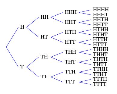
Flip the coin four times and record the outcomes. Figure 2 enumerates the sixteen different ways that these four tosses can play out. Each sequence shown has probability 1/16 of happening. Six out of sixteen have Heads and Tails in equal numbers. Four out of sixteen have three Heads and one Tail, but this is balanced by four other sequences having one Head and three Tails. One sequence has four Heads, but this is balanced by one other sequence with four Tails.
We can restate these results in terms which are independent of the sequence length. This is done by dividing sequence counts by the total number of sequences (16) while dividing the count of heads by the sequence length (4). Thus a sequence in Figure 2 can result in 0/4 = 0% Heads (4 Tails), 1/4 = 25% Heads (3 Tails), 2/4 = 50% Heads (2 Tails), 3/4 = 75% heads (1 Tail), or 4/4 = 100% Heads (no Tails). Expressed this way, 6 out of 16 = 37.5% of sequences in Figure 2 lead to 50% heads, but only 1 out of 16 = 1/16 = 6.25% of sequences lead to 100% Heads; likewise only 6.25% of sequences lead to 0% Heads (100% Tails). In all 14 out of 16 = 87.5% of sequences lead to some mixture of heads and tails (25%, 50%, or 75%) while only 2 out of 16 = 12.5 of sequence lead to unbroken runs.
Now consider what happens when the number of coin tosses increases from 4 to 8 tosses. This sequence length results in a total of 256 sequences, with outcomes narrowing from increments of 1/4=25% for 4 tosses (0/4, 1/4, 2/4, 3/4, 4/4) to increments of 1/8=12.5% for 8 tosses (0/8, 1/8, 2/8, ..., 7/8, 8/8). 238/256 ≈ 93% of these 8-toss sequences produce outcomes in the range (25%, 37.5%, 50%, 62.5%, 75%) while the remaining 18/256 ≈ 7% produce outcomes outside this range (one sequence produces 0% Heads, eight sequences produce 12.4% Heads, eight sequences produce 87.5% Heads, and one sequence produces 100% Heads). Thus the concentration of sequence counts producing outcomes in the range from 25% Heads to 75% Heads increases from 87.5% to 93%, which is what the Law of Large Numbers indicates should happen.
| Tosses | Sequences | From 3/8 to 5/8 | From 7/16 to 9/16 | From 15/32 to 17/32 |
|---|---|---|---|---|
| 4 | 16 | 37.5% | 37.5% | 37.5% |
| 8 | 256 | 71.1% | 27.3% | 27.3% |
| 16 | 65,536 | 79.0% | 54.6% | 19.6% |
| 32 | 4,294,967,296 | 89.0% | 62.3% | 40.3% |
Table 1 summarizes results obtained by taking the enumeration algorithm used to generate Figure 2 and extending this algorithm to sequences of 4, 8, 16, and 32 tosses. Remember that the discussion up to now set a very liberal standard by fixing the range 1/2±1/4 (1/4 to 3/4), by accepting sequences with outcomes in this range, and by rejecting sequences with outcomes outside this range. In Table 1 the standard tightens to the range 1/2±1/8 (3/8 to 5/8), tightens again to 1/2±1/16 (7/16 to 9/16), and tightens a third time to 1/2±1/32 (15/32 to 17/32). Thus each row of the table shows that when the number of tosses holds fast while the standards tighten, then the percent of 'acceptable' sequences declines. As would be expected. The Law of Large Numbers manifests in the columns of Table 1, where the percent advances as the number of tosses increases.
Bear in mind that this discussion of the Law of Large Numbers has entirely concerned itself with coin-toss sequences and that probability has entered into it only in the observation that every distinct sequence of Heads and Tails is equally likely as every other distinct sequence.
Uniformity
The Java documentation for java.util.Random.nextDouble() says that the method returns a
"uniformly distributed double value between 0.0 and 1.0". The word "uniform" in this description means spread equally, in the sense that 1000 calls to
nextDouble() will produce approximately 250 values between 0.00 and 0.25, approximately 250 values between
0.25 and 0.50, approximately 250 values between 0.50 and 0.75, and approximately 250 values between 0.75 and 1.00.
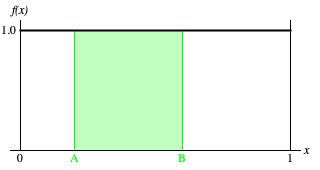
Figure 3: Graph of probability density function for the continuous uniform distribution ranging from zero to one.
The probability distribution corresponding this description is the constant function f(x)=1
over the continuous range from zero to one. Understand that this is a density function and that the probability that nextDouble()
will match any specific double-precision value is infinitesimal. Rather
think of the green region of Figure 3, a region extending from A to B,
where 0≤A<B≤1. The area of this region,
gives the probability that nextDouble() will return some value in the range from A to B.
This probability can never be smaller than zero (impossibility), which happens when A = B.
It can never be larger than unity (certainty), which happens when A = 0 and B = 1.
Recall how the Law of Large Numbers distinguished the ideal probability density function from the actual outcomes from
a random experiment. The density function graphed in Figure 3 is the ideal; however, refer back to Figure 1
to see that actual sequences generated using 32 consecutive calls to Random.nextDouble()
by no means resemble a straight (in this case vertical) line running from zero to one.
The Linear Congruence Formula must be uniform over the long term because it is cyclic. After a finite (but very large) number of iterations, the formula must ultimately repeat a value it had previously generated. At the point of repetition, the formula must do exactly what it did before. The fact that the formula works specifically with unsigned 64-bit integer variables is the constraint which ultimately forces the formula repeat itself.
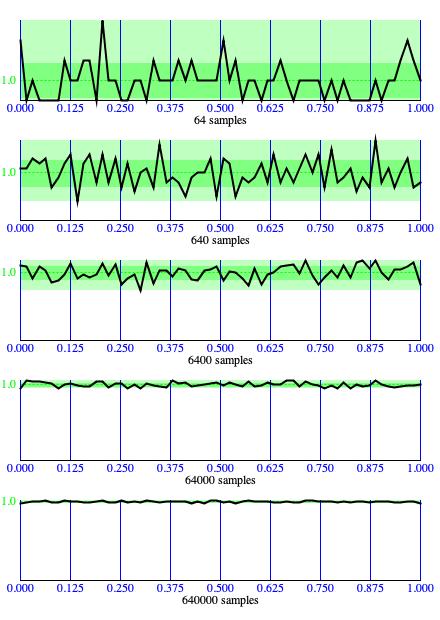
Figure 4: As population sizes increase, histograms generated by
Random.nextDouble()
conform more and more closely to ideal uniformity.
The Javamex tutorial on
java.util.Random asserts that output from Java's linear congruence implementation cycles with
a period of some 280 billion iterations. Javamex also asserts that "every possible value between 0 and [248-1]
inclusive is generated before the pattern repeats itself." Understand that this comment describes the raw linear congruence output. It does not
actually mean that single values presented by the generator
never repeat within the same cycle, since the values presented are cropped down from the 48-bit values generated
internally by the formula. It does mean that over one cycle of 280 billion iterations,
each cropped value will occur exactly the same number of times as any other cropped value.
When a particular value recurs in the same cycle, the ways that value is approached
and departed will vary from occurrence to occurrence. For examples:
-
Over one full cycle,
Random.nextBoolean()will generatetrue140 billion times andfalse140 billion times. -
Likewise over one full cycle,
Random.nextInt(280)will produce around a billion 0's, around a billion 1's, around a billion 2's, and so forth up to around a billion instances of 279.
Figure 1 showed us that sequences generated by Random.nextDouble()
can be decidedly nonuniform over the short term; however, the cyclic nature of the Linear Congruence Formula tells us that over 280 billion iterations, all
long integer values will be represented equally. The question is, does the Law of Large Numbers act upon deterministic Linear Congruence
numbers the same way it acts upon random numbers. The panel of five graphs in Figure 4 demonstrates that this is indeed the case. Each
graph in Figure 4 is a histogram: the range from zero to unity is divided into 64 regions; tallies
are maintained for each region, so that when a sample generated by Random.nextDouble()
falls into a region, the tally corresponding to that region increments.
Histogram tallies are scaled so that the largest tally extends to the full vertical height of the graph. The dashed green horizontal line plotted for y=1.0 recognizes the fact that for every 64 samples generated, an average of one sample falls in each histogram region. The darker green band identifies the range from one standard deviation below the y=1.0 line to one standard deviation above the line. 68% of region tallies fall within this darker band. The paler green band identifies the range between the minimum tally and the maximum tally. 100% of region tallies fall within this paler band.
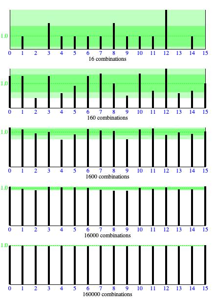
Figure 5: Each vertical bar in one of these histograms corresponds to one of the outcomes for 4 coin flips shown in the rightmost column of Figure 2 ranging from TTTT on the left to HHHH on the right. Outcomes were formed by calling
Random.nextBoolean() four times, where
true is taken as Heads and false is taken as Tails.Independence of Bit 1
The idea that each outcome in a chain of random experiments should be independent of previous outcomes is most simply
illustrated in Figure 1 where equal likelihood of Heads and Tails leads to sixteen possible
sequences from four consecutive coin tosses, all equally likely. A first verification that Java's linear congruence formula
actually behaves randomly would therefore be to use java.util.Random to generate
a sequence of Heads/Tails values, to divide this sequence into quartets of four consecutive tosses, to count how many times
each of the patterns enumerated in Figure 1 occur, and to see whether the counts are roughly equal, hence
uniform, or not.
There are various ways to simulate a coin toss using Java's Random class.
These include:
- Set a
booleanvalueq = Random.nextBoolean(). Select Heads ifqistrue, and select Tails ifqisfalse. - Set an
integervaluek = Random.nextInt(2). Select Heads ifk = 1(set) and select Tails ifk = 0(clear). - Set a
doublevalueu = Random.nextDouble(). Select Heads ifu ≥ 0.5and by select Tails otherwise. - Set a
doublevalueu = Random.nextDouble(). Set anintegervaluekto the most significant bit ofuright of the binary point. The most significant bit can be extracted by shifting the bits ofuleftward one position (multiplyinguby 2), then throwing out all bits right of the binary point (converting thedoubleexpression2.0*uto theintegervariablek). Select Heads ifk = 1(set) and select Tails ifk = 0(clear).
In practice, these alternative approaches come down to the same thing.
I ran the verification scheme just described, and repeated the run for increasingly long sequence lengths. Figure 5 presents the results. Each horizontal bar graph presents the results of one run. The numbers 0-15 below each vertical bar identify the 4-toss combinations shown in Figure 1: 0 is the top-listed combination HHHH, 1 is the second-listed combination HHHT, and so forth. Where the legend says "16 samples", that means 16 coin-toss quartets were generated. Four of the combinations listed in Figure 1 where not present in this data. Nine combinations happened once only. Two combinations happened twice. One combination recurred three times.
Had each combination appeared exactly once in the "16 combinations" graph, that would have been suspicious. It would have suggested that some agency was intervening to make sure each combination got its 'fair share' over the frame.
Moving one step down to the "160 combinations" graph, the distribution of combinations remains decidedly non-uniform, though no other distribution suggests itself.
Continuing down through increasingly large sample counts, one sees the distance from the largest combination tally to the smallest combination tally tighten up — relative to the overall sample count. The "1600 combinations" graph is arguably uniform, and the "16000 samples" graph is decidedly so. With "160000 combinations" the band of deviation becomes to narrow to plot.
Independence of Bits 1-4
When Donald Knuth examined the question of "What is a random sequence?", he concluded that a generator is maximally independent when all sequences (orderings) of values are equally likely.2
Knuth goes on to describe various ways of testing whether a sequence is random, most famous being the spectral test. (You can find an updated list in Wikipedia's article on Statistical Randomness.) Knuth's cauched his descriptions in hypothesis-testing terms; that is, each test assumes that the sequence is dependent in some way, and the test looks for behavior that is characteristic of that particular flavor of dependence.
It seems to me that these look-for-dependency tests go at the question indirectly when Knuth himself has provided a criterion that can be verified directly, at least up to a limit. To understand this limit, it is necessary to understand that any real value in the range from zero to unity can be expressed in fixed-point binary form, where every bit left of the binary point is zero. The most significant bit (MSB) to the right of the binary point determines whether the value falls in the interval from 0.0 to 0.5 (MSB clear) or falls in the interval from 0.5 to 1.0 (MSB set). The two most significant bits to the right of the binary point determine whether the value falls in the interval from 0.00 to 0.25 (00), the interval from 0.25 to 0.50 (01), the interval from 0.50 to 0.75 (10), or the interval from 0.75 to 1.00 (11). Likewise the most significant nibble (4 bits) divides the range into 16 intervals, each of width 1/16=0.0625.
Figure 5 previously demonstrated that the criterion of independence is satisfied for the most signficant bit. This can be interpreted graphically in terms of sequence values appearing either in the lower range from 0.0 to 0.5 or the upper range from 0.5 to 1.0.
How can we verify that Random.nextDouble()
produces independent values? It is feasible to cleave the most significant bits right of
the binary point () and verify that these at least are independent. Take the 4 most
significant bits in particular. 4 bits (one nibble) is capable of dividing the range from
zero to unity into 16 parts. Let u1, u2, …, uk-1,
uk, …, uN be a sequence of values generated by
Random.nextDouble().
Independence means that the value taken by uk-1, has no effect whatsoever upon the likelihood
that uk will fall into any particular part. Uniformity means that all 16 parts have equal likelihood,
i.e. 1/16. The paths for 4-bit values branch out somewhat like Figure 1, except that instead of each path dividing
into 2 sequences with each additional coin toss, the paths for 4-bit values divide into 16 separate sequences for each additional sequence element.
Thus there are 16×16=256 ways of forming sequences of 2 4-bit values, 16×16×16=4096 ways of forming sequences of 3 4-bit
values, and 16×16×16×16=65536 ways of forming quartets of 4-bit values.
That's way too many values to present graphically as histogram bars. Allocating an array of 65536
long-integer tallies would have been challenging for mainframe computers in
Donald Knuth's time, but it is no problem at all for today's virtual-memory desktop models.
I set up such an array of 65536 tallies to count nibble quartets. Packing four nibble values into the low 16 bits of an
int gave me a nibble-quartet ID ranging from 0 to 65535. Every 16-bit integer
in this range identifies a specific quartet, and all distinct quartets are accounted for. So this 16-bit integer provided an index
into the array of tallies.
I generated sequences using Random.nextDouble(),
resolved each double value into a 4-bit nibble (multiply by 16., then truncate to the next lower integer), and gathered the nibbles
into quartets. I formed an index from each quartet's nibbles and incremented the tally corresponding to that index. The results of this effort are summarized in
Table 2. Having too much data to evaluate graphically, it is necessary to rely on numerical expressions of the green
bands in Figure 4 and Figure 5: the paler green "range" band is
expressed in the Diff/Avg column, while the darker green "standard deviation" band is expressed in the
Dev/Avg column.
Random.nextDouble(),
resolved to 4 significant bits,and gathered into quartets.
The quartet counts in column 1 of Table 2 were selected so that the average number of times each combination happened (column 2) would be a power of 10. After 35536 quartets, enough had been generated to represent each combination once, but that is not what happened. Some combinations never happened (column 3), while others recurred as many as 8 times (column 4).
If the combination tallies even out as quartet counts increase, this will tell us that every combination is equally likely over the long term. If every combination is equally likely over the long term, then nibble independence is verified. But we can't lay out 65536 nibble-quartet tallies as vertical bars the way 16 coin-toss quartet tallies were laid out in Figure 5. What is required is some way of measuring how closely the individual tallies cluster around the average. Tallies closing in toward the average means nibble independence. Not closing in means that some combinations are favored over others — that is, nibble dependence.
Table 2 measures clustering around the average in two ways, one coarse and simple, the other finer, complicated, and statistically orthodox.
- The coarse measurement presented as Diff in Table 2 (column 5) subtracts the smallest tally from the largest tally. This measurement is the numerical counterpart to the paler green bands in Figure 4 and Figure 5. Interpreted statistically, the minimum and maximum tallies together define a range within which 100% of instances will reside.
-
The finer measurement presented as Std Dev in Table 2 (column 7) is called the
standard deviation.
This measurement is the numerical counterpart to the darker green bands in Figure 4 and Figure 5.
It is calculated using this formula:
Std Dev = √ 1 N ΣN-1 k=0 (Tallyk - Avg)2
Compared to the max-min difference, the standard deviation gives a more intuitive measure of how 'run-of-the-mill' tallies cluster around the average. In Table 2 the ranges from one standard deviation below average to one standard deviation above average are about a quarter of the distances from the minimum tally to the maximum tally.
Neither the Diff measure nor the Std Dev measure reduces toward zero as quartet counts increase; however when normalized relative to the average number of instances per combination (Diff/Avg, column 6; Dev/Avg, column 8), the evening-out effect of growing populations is indisputable.
For most applications, uniformity and independence are the two behaviors that matter more even than actual indeterminacy. The present discussion has at this point established two tests, initially graphic but ultimately quantitative, one for uniformity and one for 4-bit independence. These tests work straight from the premises that sequence values (for the uniformity test) and quartets of sequence values (for the independence test) should be equally likely. While passing these tests does not prove randomness, failing them does prove unsuitability.
Seeding the Random Generator
As just explained, Java's linear congruence generator internally iterates through [248-1] (≈ 280 billion) 48-bit values before returning to its original value and thus repeating the cycle. It's pretty hard for an application to burn through [248-1] values. For most applications the length of random sequences rarely extends beyond a few thousand. Of greater concern is the ability to present the same sequence each time the application executes or, alternatively, to present a different sequence each time.
The method used to determine where to start in this cycle of 280 billion values is Random.setSeed(),
which accepts a single long integer argument supplying the initial value X0 for the linear congruence formula. Understand
that the formula intervenes after the call to Random.setSeed() and before the return from
Random.next().
If the application uses random data for test purposes and the test fails, then the developer will want to identify the point of failure, correct the application, and retry the test. In such a context one would want to reproduce the conditions which led the previous test to fail, so it makes sense that both test and retest employ the same seed.
For applications such as gaming or muzak generation, one would want each run of the application to produce a different experience. Here it makes sense acquire a random seed from
some outside source. You could, perhaps, request a seed value from the operator. A more common approach is to sample the system clock, as illustrated in
Listing 1. Oracle's Java platform documentation for
System.currentTimeMillis()
explains that currentTimeMillis() returns "the difference, measured in milliseconds, between the current time and midnight, January 1, 1970 UTC."
A practice which I saw once in a book (but which I have since been unable to track down) reseeds the random generator from the system clock each time a random value is generated. Listing 2 illustrates a wrapping class which does this. No justification was given for this practice, which invalidates all arguments and demonstrations so far given for the uniformity and independence of sequences generated using the linear congruence formula. The effect of linear congruence in this instance is to spatter what would be an ascending sequence of timing values all over the range from zero to unity.
Seeding the random generator once is imperative, but seeding it more than once is pointless. Java's Random class has
already been demonstrated to satisfy both the criterion of uniformity and the criterion of independence. What greater benefit could be obtained?
Still, having developed histogram tests of these two criteria, I am curious to know whether these developers did themselves actual damage. If you
are less curious, you should probably skip ahead to the next topic.
The next step is to apply the two tests developed in this presentation, the uniformity test and the 4-bit independence test
One challenge faced in testing iterative reseeds is that I do not have knowledge of the timing context under which the iteratively reseeded generator was
called. Presumably the original context was a real-time control scenario, where durations on the order of a second or larger elapsed
between each call. If I run direct tests iterating calls to ReseededRandom.nextDouble(),
many consecutive calls will happen within the same millisecond, and the returned values will hold constant over these time intervals.
A comprimise might be to reseed only when the system clock value changes, letting the generator
iterate while the system clock value holds constant. However, this compromise strays from the always-ascending profile offered by
successive calls to currentTimeMillis().
Such a profile could be had by dispensing with timing and simply iterating seed values: 1, 2, 3, 4, and so forth.
However, the linear congruence formula reponds to each input with a distinct output until the input reaches 248-1, then cycles all over again.
So that's just repeating the cycle in a different order.
Sharing the Random Generator
Suppose you're building a composing program which generates several simultaneous voices, and you want each voice to exhibit
behavior which is uninfluenced by what any other voice is doing. Alternatively, you're building an animation program which depicts
several goats, and you want each goat to wander independently. In either case, suppose the actors in each scenario go along until a decision
point comes along, and that decision relies to some extent upon generating a random number. How do you implement the random component? Do you create
a separate Random instance for each actor (call this Option A) and somehow contrive to seed each
Random instance independently? Or do you simply instantiate Random
once (call this Option B), seed the single instance from the system clock, and share the one generator between all actors?
We already know that the various sequences generated using Option A will be suitably uniform over the long term
and suitably indpendent over the short term. Option B is clearly simpler, but can the same assertions be made of sequences drawn from one
shared generator? I have set up a test
to determine whether this is so. There a two Random instances, each seeded differently.
One Random instance serves as the shared random generator, producing values through
Random.nextDouble(). The second
Random instance distributes sequence elements to actors P,
Q, R, and S based
on values produced by Random.nextInt(4).
The first question is, are the values in the P, Q, R, and S subsequences distributed uniformly between zero and unity? Table 3 addresses this first question. The table replicates the format of Table 2 for the four sample sets. Having 16 possible nibble values, it is appropriate to divide the range from zero to unity into 16 intervals. Presented graphically, the histograms would resemble those in Figure 5, except that those were about independence and these are about uniformity. Having the coarse and finer numerical measures for how tally counts disperse around the norm, and not always having the luxury going forward to use graphs (since the histogram bars will often be too numerous to graph), this presentation will limit itself to numbers going forward.
Pay particular notice to the Count, Avg, and Dev/Avg (normalized standard deviation) columns for each sample set. We shouldn't expect uniformity when the Samples total is 64 (16 samples per subsequence stream, averaging 1 sample per histogram bar) or 640 (10 samples per histogram bar). For a Samples total of 6400, the process described allocated 1599 samples to subsequence P, 1608 samples to subsequence Q, 1621 samples to subsequence R, and 1572 samples to subsequence S. These counts provided the opportunity for each sequence to manifest each distinct nibble value 6400/4/16=100 times per histogram bar — actual averages vary within 2% of this ideal. However the stats that really matter are the normalized standard deviations (Dev/Avg); these values are 0.141, 0.112, 0.085, and 0.121 — all under 15%. Increasing the number of samples by 10 drops the normalized deviations down to under 4%.
| P | Q | R | S | |||||||||||||||||||||||||||||
|---|---|---|---|---|---|---|---|---|---|---|---|---|---|---|---|---|---|---|---|---|---|---|---|---|---|---|---|---|---|---|---|---|
| Samples | Count | Avg | Min | Max | Diff | Diff/Avg | Std Dev | Dev/Avg | Count | Avg | Min | Max | Diff | Diff/Avg | Std Dev | Dev/Avg | Count | Avg | Min | Max | Diff | Diff/Avg | Std Dev | Dev/Avg | Count | Avg | Min | Max | Diff | Diff/Avg | Std Dev | Dev/Avg |
| 64 | 13 | 0.812 | 0 | 2 | 2 | 2.462 | 0.808 | 0.994 | 17 | 1.062 | 0 | 5 | 5 | 4.706 | 1.298 | 1.221 | 17 | 1.062 | 0 | 3 | 3 | 2.824 | 0.747 | 0.703 | 17 | 1.062 | 0 | 3 | 3 | 2.824 | 1.088 | 1.024 |
| 640 | 167 | 10.438 | 5 | 16 | 11 | 1.054 | 3.201 | 0.307 | 163 | 10.188 | 5 | 19 | 14 | 1.374 | 3.575 | 0.351 | 150 | 9.375 | 4 | 14 | 10 | 1.067 | 3.276 | 0.349 | 160 | 10.000 | 5 | 14 | 9 | 0.900 | 2.208 | 0.221 |
| 6400 | 1599 | 99.938 | 81 | 122 | 41 | 0.410 | 14.091 | 0.141 | 1608 | 100.500 | 80 | 120 | 40 | 0.398 | 11.258 | 0.112 | 1621 | 101.312 | 82 | 113 | 31 | 0.306 | 8.600 | 0.085 | 1572 | 98.250 | 80 | 124 | 44 | 0.448 | 11.845 | 0.121 |
| 64000 | 16009 | 1000.562 | 942 | 1081 | 139 | 0.139 | 36.971 | 0.037 | 15988 | 999.250 | 931 | 1061 | 130 | 0.130 | 36.108 | 0.036 | 16008 | 1000.500 | 941 | 1073 | 132 | 0.132 | 35.709 | 0.036 | 15995 | 999.688 | 944 | 1043 | 99 | 0.099 | 24.619 | 0.025 |
| 640000 | 159508 | 9969.250 | 9794 | 10059 | 265 | 0.027 | 74.395 | 0.007 | 160261 | 10016.312 | 9827 | 10173 | 346 | 0.035 | 113.857 | 0.011 | 160362 | 10022.625 | 9869 | 10216 | 347 | 0.035 | 84.619 | 0.008 | 159869 | 9991.812 | 9854 | 10211 | 357 | 0.036 | 105.486 | 0.011 |
Random.nextDouble() values shared out between 4 subsequences.The second question is, are the values in the P, Q, R, and S sequences individually independent? Table 4 addresses this second question. There are 164=65536 distinct sequences which can be formed of 4-bit integers, taken 4 in a row. The first row of Table 4 shows results for 1,048,576 Samples overall. The four most significant bits of these samples are gathered into 4-member quartets, giving 1,048,576/4=262,1444 Quartets overall. Distributing these quartets among the P, Q, R and S sequences gives 262,1444/4=65536 quartets per sequence, and the opportunity for each distinct quartet to be represented one time. In practice, some quartets aren't represented at all, while quartets recurred as many as 7 or 8 times depending which subsequence you're drilling down into: P, Q, R, or S.
We would not expect quartet counts to be uniform with only one quartet-candidate per tally. However, moving down to the third row of the table there are 104,857,600 Samples overall giving 100 quartet-candidates on average per distinct sequence. The normalized standard deviations in this row all come in at 10%; in the next row down they come in at 3%.
| P | Q | R | S | ||||||||||||||||||||||||||||||
|---|---|---|---|---|---|---|---|---|---|---|---|---|---|---|---|---|---|---|---|---|---|---|---|---|---|---|---|---|---|---|---|---|---|
| Samples | Quartets | Count | Avg | Min | Max | Diff | Diff/Avg | Std Dev | Dev/Avg | Count | Avg | Min | Max | Diff | Diff/Avg | Std Dev | Dev/Avg | Count | Avg | Min | Max | Diff | Diff/Avg | Std Dev | Dev/Avg | Count | Avg | Min | Max | Diff | Diff/Avg | Std Dev | Dev/Avg |
| 1048576 | 262144 | 65473 | 0.999 | 0 | 8 | 8 | 8.008 | 0.998 | 0.999 | 65649 | 1.002 | 0 | 8 | 8 | 7.986 | 0.999 | 0.997 | 65744 | 1.003 | 0 | 7 | 7 | 6.978 | 1.002 | 0.999 | 65277 | 0.996 | 0 | 8 | 8 | 8.032 | 1.001 | 1.005 |
| 10485760 | 2621440 | 654940 | 9.994 | 0 | 25 | 25 | 2.502 | 3.165 | 0.317 | 655667 | 10.005 | 0 | 25 | 25 | 2.499 | 3.170 | 0.317 | 655771 | 10.006 | 0 | 27 | 27 | 2.698 | 3.161 | 0.316 | 655061 | 9.995 | 0 | 29 | 29 | 2.901 | 3.170 | 0.317 |
| 104857600 | 26214400 | 6554068 | 100.007 | 61 | 147 | 86 | 0.860 | 10.047 | 0.100 | 6553926 | 100.005 | 62 | 152 | 90 | 0.900 | 10.034 | 0.100 | 6555926 | 100.035 | 58 | 146 | 88 | 0.880 | 10.037 | 0.100 | 6550479 | 99.952 | 59 | 148 | 89 | 0.890 | 9.985 | 0.100 |
| 1048576000 | 262144000 | 65536807 | 1000.012 | 875 | 1129 | 254 | 0.254 | 31.675 | 0.032 | 65531334 | 999.929 | 870 | 1165 | 295 | 0.295 | 31.541 | 0.032 | 65541317 | 1000.081 | 869 | 1140 | 271 | 0.271 | 31.754 | 0.032 | 65534540 | 999.978 | 868 | 1138 | 270 | 0.270 | 31.785 | 0.032 |
Random.nextDouble() values shared out between 4 subsequences.Random Shuffling
Jacob Bernoulli, the original probability theorist, explained probability using an urn model. This model placed colored pebbles in an urn, then drew one or more pebbles blindly from the urn. For example, if the urn contained six white pebbles and four black pebbles then the probability of choosing a white pebble would be 6 out of 10. The urn model extended beyond single trials to consider random sequences, and it investigated the difference between selection with replacement, where the proportions of colors remains fixed, and selection without replacement, where extracting a pebble affects the mixture remaining.
Random shuffling takes selection without replacement to exhaustion. Shuffling is a kind of permutation in that it arranges the members of a population into a particular order. The number of possible ways of arranging a population with N members may be calculated as "N factorial" (symbolized N!):
For random shuffling, each arrangement is just as likely as every other arrangement. Although the term "shuffling" originally derives from the actions that card players take to mix up their decks, those actions typically do not randomize as thoroughly as selection without replacement would do.
Random shuffling eliminates all bias from the order in which members of a population are presented. Within computer programs, populations are typically generated using an enumeration algorithm; for example, by feeding equally spaced driver values through a statistical transform. This particular approach lists populations in ascending range order, which random shuffling will counter. The combination of tailored population generation plus shuffling is an effective way to conform a frame of choices as precisely as possible to a chosen distribution.
The random shuffling algorithm provided below in Listing 1 implements selection without replacement. It is good for obtaining
totally unbiased orderings, but what if you want to promote certain tendencies while still eliminating any influence from the enumeration algorithm?
The answer to this qualified circumstance is developing a preference value with integer and fractional parts. Suppose you're writing a program for
musical part writing, it has just completed one chord and it is now time to choose the order of voices for composing the next chord. First priority goes to
the voice that needs to resolve a dissonance; give that voice an integer preference value of 8. Second priority goes to the voice that needs to satisfy a leading tone; give
that voice an integer preference value of 4. Third priority goes to the bass voice; if that voice does not satisfy priorities 1 or 2, give that voice an integer
preference value of 1. All remaining voices get an integer preference value of 0. To eliminate bias due to the algorithm for enumerating voices, use
Random.nextDouble() to supply the fractional part of the
preference value. Then sort the voices by preference. Notice that the
SharedRandomGenerator implementation class.
Singleton Coding
The SharedRandomGenerator detailed in Listing 1 does not in any way attempt to supercede Java's built-in
Random class. Rather it wraps one instance of Random within a
class that allows simultaneous sequence-generating processes to draw upon one single random source,
which source only needs seeding once during any particular run of a program. Seeding in one place is most definitely a great convenience.
While the previous section on
"Seeding the Random Generator" did not show that reseeding the generator before each call necessarily violated the criteria of uniformity and/or
independence, the fact that Random already manifests these characteristics renders iterative seedings pointless.
Since "Sharing the Random Generator" demonstrated that the sub-sequences resulting when several different processes
call out to the same Random instance will themselves be both uniform and independent, this practice
is a good one.
The guts of the SharedRandomGenerator provide a textbook implementation of the
singleton design pattern. There's a private and
static variable named
singleton which holds the only SharedRandomGenerator
instance.
There's a static getSingleton() method whose first call instantiates
singleton and whose latter calls always give back the same instance. The class
constructor is private so that only getSingleton()
can instantiate SharedRandomGenerator instances.
The SharedRandomGenerator class is as simple as they come. It contains just one property, the single
instance of java.util.Random. This property has no setter, being initialized in the constructor. It is
accessible only by getRandom(), the getter. You can seed this Random
instance directly or employ the SharedRandomGenerator class's
setSeed() method. SharedRandomGenerator.setSeed()
only permits itself to be called one time.
The SharedRandomGenerator class is enhanced by two static shuffle()
methods implementing the Fisher-Yates shuffling algorithm. This algorithm is
ultimately due to Bernoulli, since it directly implements selection without replacement; it came to me by way of
Donald Knuth's Seminumerical Algorithms.
One shuffle() operates on Object arrays; the other operates on collections
implementing the java.util.List
interface. These methods aren't just included within the SharedRandomGenerator class for convenience. They fully leverage
the shared Random
instance. Thus seeding Random also seeds these shuffles.
Comments
- The primary source for this page was Chapter 3, “Random Numbers” in Donald Knuth's Seminumerical Algorithms. Knuth remains excellent for his treatment of Derrick Henry Lehmer's “linear congruence” algorithm, the method universally used today. Linear congruence produces number sequences which satisfy all characteristics of unpredictability, but only for the uniform case. The only two non-uniform cases dealt with by Knuth were the "polar" method of generating bell-curve randomness and a method for generating negative-exponential values. The "polar" method is a dead end because it inextricably intermingles randomness with distribution. The method for generating negative-exponential samples (the same method used by Xenakis) was more promising because it separated an active step from a passive step. The active step used linear congruence to generate random decimal number uniformly in the range from zero to unity. The passive step applied a mathematical function which mapped the linear congruence values into the range from zero to infinity with densities trending to zero as values increased.
- The present text is adapted from my Leonardo Music Journal article from 1992, "A Catalog of Sequence Generators". The headings are "Independence (Randomness)", p. 56, and "Lehmer's 'Linear Congruence' Formula", p. 58.
- The passage cited appears in "Random Numbers", Chapter 3 of Seminumerical Algorithms, p. 127. I gleaned the subsequent insight during the 1970's but reading through Knuth today have been unable to locate the exact turn of phrase which inspired it.
| © Charles Ames | Page created: 2022-08-29 | Last updated: 2022-08-29 |