Basics II: Distributions

Introduction

A distribution is a way of summarizing the content of a population. Statisticians generally start with a population, then seek to determine which distribution fits best. However, the Transform component of the Driver/Transform pattern for sequence generation goes somewhat the other way: It starts with a distribution and uses it to shape the intermediate output from the Driver component, whose values presumably are uniform.

Rarely will the shaping distribution will be representable using an explicit mathematical formula such as the familiar bell curve. More common alternatives include the composition of the orchestra in Xenakis's Stochastic Music Program, where the probability density for each timbre selection is a number calculated in response to the current section density. Whether formulaic or numeric, the discipline of probability theory provides the mathematical constructs necessary both to describe the distribution (the probability density function or PDF) and to transform uniform Driver values so that the results conform to said distribution (by inverting the cumulative density function or CDF). This page and its dependents explain how to make these mathematical constructs functional as DistributionBase subclasses. The distribution classes can be used outright, but they can also be leveraged by Transform classes when no closed-form inverse-CDF formula exists (the common situation).

But first. There's some terminology associated with the distribution concept, and the best way to explain the terms is with reference to an example taken from the statistician's perspective. Hence Figure 1.

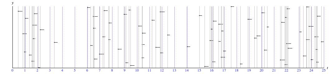
Figure 1: A sequence of events emulating the Poisson Point Process.

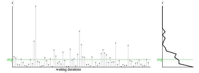
Figure 2: Durations waiting between consecutive events from Figure 1.
Left — Waiting duration detail. Right — Continuous histogram.

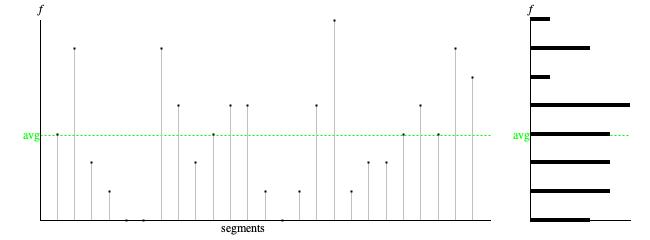
Figure 3: Event counts by segment from Figure 1.
Left — Event count detail. Right — Discrete histogram.

Figure 1 shows the kind of situation which distributions can be helpful in summarizing. It in fact illustrates a Poisson Point Process, which is a scenario developed by probability theorists to model the experience of waiting for something to happen.¹ Xenakis was familiar with this scenario; his Stochastic Music Program models both section durations and note-to-note waiting durations as Poisson Point Processes.

• The horizontal axis, labeled t in Figure 1, represents time.
• The small black dots with line-segment 'tails' indicate events which happen over time.
• The vertical placement of events (y axis) is there simply to help distinguish events from each other.
• The non-dashed vertical gray lines help pinpoint the relative timing of events.
• The dashed vertical blue lines measure out units of time, which could be minutes, hours, days, years, ….
• Had Figure 1 been about fishing on a lake ("poisson" is French for "fish"), the length of an event's tail might be taken to indicate the size of the fish just caught. But it's not about that. The 'tails' simply render events more noticeable.

Taking a mass of data and boiling it down is the heavy lift of most statistical analysis. The Poisson Point Process treats two complementary domains (perspectives) in modeling situations like Figure 1, the time domain and the frequency domain. The time domain models the durations spent waiting between consecutive events. The frequency domain models how many events happen over each unit of time.

Figure 1 has 74 events but 75 waiting durations dispersed along 25 time units. At the highest level of summary, a statistician could calculate two averages: the average waiting duration (25/75=0.333) for the time domain, and the average number of events per time unit (74/25=2.960) for the frequency domain. These numbers may be very useful, but only to a point. They give no insight into the spread of larger and smaller values. Further summary statistics (e.g. standard deviation) can account for the spread, but for most of us its more insightful to determine the range of values, to identify where values are most concentrated within the range, and to identify where values are more sparse. In other words, we want to know the distribution.

Of the two complementary perspectives, the time-domain perspective involves the sequence of 75 samples detailed in the leftward graph of Figure 2. Remember that sequence is a population presented in one specific order. Since these clock-time durations have digits right of the decimal point, we characterize the range of sample values as continuous and represent them using the Java datatype double.

• The time-series graph presented leftward of Figure 2 plots individual waiting durations by order of occurance. The sample values in this sequence range from 0.001 (just above the horizontal axis) to 2.670 at the topmost position. The average value of 0.333 is plotted horizontally as a dashed green line.
• The "continuous histogram" presented as the rightward graph of Figure 2 was constructed by dividing the vertical range from zero to 2.670 into 20 vertical intervals, by counting up the number of sample values in each Confidence_interval, by plotting the counts left aligned, then connecting the plotted points with straight lines. The resulting curve closely resembles a negative exponential distribution, which is what the Poisson point process predicts.

The frequency-domain perspective involves the sequence of 25 segments detailed in the leftward graph of Figure 3. Since these event counts never have digits right of the decimal point, we characterize the range of sample values as discrete and represent them using the Java datatype int.

• The time-series graph presented leftward of Figure 3 plots event counts per segment by segment order. The sample values for this frequency-domain sequence range from 0 (inclusive) to 7. The average value of 2.960 is plotted horizontally as a dashed green line.
• The "discrete histogram" presented as the rightward graph of Figure 3 was constructed as a bar graph showing how many of the 25 time units had no events (bottommost bar), how many time units had one event (next-to-bottommost bar), and so forth up to 7 events (topmost bar). The distribution which the Poisson point process predicts for event counts in a time period is known formally as the Poisson distribution; its main feature is a hump around the average, tapering down to a smaller positive density for zero events, and tapering down to zero as event counts rise. The bar graph rightward of Figure 3 conforms to this description, though the shape is less elegant than the ideal graphs shown in Wikipedia.

An important thing to understand about statistical distributions is that while many distributions are motivated by probability theory, probability does not figure in the fundamental nature of the concept. A distribution describes characteristics of a population whose size is abstracted as unity (100%). The describing focuses on the range of sample values, whether that range is discrete or continuous, and how sample values are weighted (high weights where values concentrate, low weights where values are sparse). No assumptions are made about the genesis of the population, which may be random, chaotic, or entirely deterministic.

Mathematical Underpinnings

Various constructs underpin the mathematical theories of probability and statistics. The notion of the probability domain provides an all-some-none ideal, while various mathematical functions (PDF, CDF, and quantile) enable us to translate back and forth between this ideal and the distribution's real-world range.

Probability

Normally in the general world of mathematics, the source set from which a function draws its input is called the domain, while the target set which receives the function's output is called the range. However, the more specialized world of probability and statistics speaks contrariwise, of functions drawing input from the range of a distribution (also called the sample space) and limiting output to the probability domain.

Probabilities are continuous. They are numbers with digits right of the decimal point (mostly zero to the left), and they represented using a floating-point datatype such as double. Probabilities run from zero to unity. Here a further bifurcation of worlds applies: In the chance world of probability theory, zero means impossibility (won't happen) while unity means certainty (always happens). However in the chance-optional world of statistics, "probability" descends from the concept of a percentage, which word has been around since Roman times. It represents a proportion of a total population: zero (0%) means nothing; unity (100%) means everything.

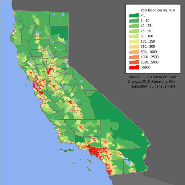
Figure 4: California population densities (from Wikimedia Commons).

Population Density

For example, Figure 4 graphs population density around the state of California. The large low-population swaths on the lower right of the graph cover features like the Mojave desert and Death Valley, The red coastal blotch in the bottom-left county is San Diego, and the next blotch up the coast is the urban sprawl covering greater Los Angeles, Orange County, and stretching eastward to San Bernardino. The coastal cluster up north comprises the Bay Area cities of San Francisco, San Jose, and Oakland. The mid-state chain includes the Central Valley cities of (proceeding southward) Sacramento, Stockton, Fresno, and Bakersfield. The orange smear in the far north, mid way between the coast and the Nevada border and surrounded by National Forests, is Redding.

It would be possible to mark off the state of California into a mile-square grid, then count the number of individuals in each square, but that is not what happens. Instead the Census Bureau divides the United States into 8,057 tracts; in urban areas these tracts divide into block groups (23,212 of those), and the block groups further divide into blocks (710,145). The numbers given here source from the Census Bureau's 2010 information page for California. The Bureau is somehow able to tie every individual's residence address (which the most important fact it collects about people) to a tract, and where they are defined, to a block group and to a block. Census tracts, block groups, and blocks are accurately mapped; the Bureau precisely knows both how each geographical region is bounded and how many square miles it encloses. Wikipedia reports that localities cooperate with the Bureau in defining tracts, groups, and blocks (originally city blocks but no longer), so that municipal boundaries are respected and populations are "homogeneous". Wikipedia also passes along the comment that each tract averages "about 4,000 inhabitants" but Wikipedia does not clarify why this average would be known before the actual census is taken. However the uniform average does imply that tracts cover smaller areas in urban locations where population is dense and larger areas in rural locations where population is sparse.

The Census Bureau thus collects data on how many individuals live in each geographical region. However comparing raw population numbers is not directly meaningful between regions of differing size. Calculating the population density is a simple matter of dividing individuals by square miles — and densities are comparable.

Census regions being singular entities, the relationship between regions and population densities is a discrete distribution, that is, a distribution over a discrete range. However the larger the number of range values covered by a discrete distribution (in this case 710,145), the closer a discrete distribution comes to resemble a continuous distribution. A glance at Figure 4 confirms this. The visual impression is not of points, but rather of a surface with high red peaks descending to low green valleys.

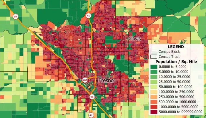
Figure 5: Census blocks in Fresno, California (from Caliper.com).

Figure 5 drills down from California statewide (Figure 4) to the city of Fresno. The image details census blocks (outlined in light gray) — which are the smallest geographical regions for which census data is collected — also their enclosing census tracts (outlined in black). Each census block defines a prism whose base is the physical area, whose height is the population density, and whose volume (base × height) is the population enclosed within the region. Since the height of the prism measures the distance from the x-y plane up the z axis to the surface forming the red peaks and green valleys, we can properly speak of calculating the population as calculating the "volume" under the population-density "surface". Calculating the volume of the whole comes down to summing the volumes of the parts; thus calculating the population of each census tract in Figure 5 comes down to summing the volumes of the census blocks that make up the tract, while calculating the population of Fresno comes down to summing the volumes of its census tracts.

Probability Density Function

The probability density function or PDF associates every sample value in the distribution's range to a probability density ranging from zero to unity. Probability densities (or just "probabilities") are population densities which have been normalized to abstract away the specific population size. For example, the 2010 population of Fresno, CA was 531,576 spread out over 112 square miles. The population density calculates as 531,576 / 112 = 4746, the probability density is that amount divided by the 2010 population of California: 4746 / 39,512,223 = 0.00012 and the probability that an individual chosen at random from the 2010 California tax rolls will reside in Fresno is 0.00012 × 112 = 0.013 or 1.3%.

A distribution is formally specified by its PDF. Summary statistics such as the mean (average) and standard deviation are contingent on the PDF, as are the CDF and quantile function described below. A PDF will be either discrete or continuous, depending on the distribution's range:

• If range of the distribution is discrete (nothing right of the decimal point), then p_k = PDF(k) where the independent variable k is an integer and the dependent variable p_k is a real number ranging from zero to unity. Each probability p_k is called a "point density", and all the probabilities sum to unity.
• If the range of the distribution is continuous (digits right of the decimal point) along a single v axis, then p = PDF(v) where the independent variable v is a real number, the dependent variable p is a non-negative real number, and the PDF itself is a continuous (no abrupt jumps), curve. The probability density p does not give the probability of selecting one particular v in the range.² Rather, the probability that the selected value v will fall in the interval from a to b is given by the area under the PDF curve from a to b. "Area under the curve" means base times average height; that is, the width of the interval times the average density during the interval. If a and b are close, then p = PDF((a+b)/2) gives a good approximation for average height. If a and b are not close, then the interval can be divided in half and half again until the section endpoints are close; the areas above these sections can be summed. The area under the entire PDF curve always equals unity.
• If the range of the distribution is continuous along both x and y axes, then p = PDF(x, y) where the independent variable (x, y) is a point on a plane, the dependent variable p is a non-negative real number, and the PDF itself is a continuous (no abrupt jumps), surface. The probability that a selected point will lie within a specific contiguous region of the plane is calculated as the volume under the PDF surface; that is, the area of the region times the average PDF value within the region.

Cumulative Distribution

The cumulative distribution function or CDF returns the probability (zero to unity) that any other sample value will be less than or equal to sample value given as input. In particular, CDF(b) - CDF(a) gives the probability that a sample value v will fall between a and b, where a < b.

I hinted previously that the CDF enriches the population-based interpretation of values in the probability domain. This insight pertains to continuous distributions along a single axis. Suppose there's a sample value v such that CDF(v) = 0.5. Then half of the population upon which the distribution is based will have values less than v, and the other half of the population will have values greater than v. But that means that v must be the average sample value. Now suppose there are two sample values: a such that CDF(a) = 0.5-0.341 and b such that CDF(b) = 0.5+0.341. Then the range from a to b embraces 0.341+0.341 = 0.682 = 68.2% of the population. When the distribution is a bell curve, this corresponds to the interval within ±1 standard deviation of the average. (The probability difference for the 2nd standard deviation reduces from 34.1 to 13.6).

Knowing the CDF is a necessary prerequisite for transforming driver values into range values (see the quantile function below). However, the concept becomes problematic when a distribution ranges continuously over an area — for example, over the state of California. It is not meaningful to say that one location is "greater" than another when both north-south and east-west axes must be taken into account. One workaround would be to calculate a separate CDF can for each axis. A second workaround would be to granularize the area, much as the Census Bureau granularizes the United States into tracts. This would transform the range of the distribution from a continuous area into a discrete collection of regions, and each region can be assigned an identification number. A CDF can work with that.

Implementing a CDF programmatically requires one simple enhancement to the collections already used to implement the PDF. That enhancement is to add a sum to each distribution item, which sum will accumulate the weight of the current item (for ContinuousDistributionItem instances, that means the trapezoidal area) with weights of all the item's predecessors. Calculating the CDF(v) for a specific sample value v first requires finding which collection item pertains to v. If the distribution is discrete, that's it. If the distribution is continuous, there's an interpolation formula which I explain on the page devoted specifically to continuous distributions.

Quantile Function

The inverse cumulative distribution function, indicated CDF^-1, is also called the quantile function. This function maps every value q in the range from zero to unity to the sample value v for which q is the proportion of sample values ≤ v. For example, if the population embraces possible scores on the PSAT, then CDF^-1(0.95) gives the score which places a student in the top 5% (95th percentile) of test takers. The population-based interpretation of the probability domain coincides with what the Driver/Transform pattern refers to as the driver domain. The range from zero to unity could alternatively be designated the quantile domain: I have not seen this term used, but it is entirely appropriate.

The quantile function is also used by statisticians to calculate confidence intervals. This is how a statistician can claim to be 90% certain of an assertion.

Inverting the CDF programatically requires no more data support than what was described for the CDF itelf. To start out, my code calculates a chooser by multiplying the driver by the total weight of all distribution items combined. The code then identifies the distribution item whose cumulative-sum-of-weights is minimally larger than or equal to the chooser. If the distribution is discrete, that's it. If the distribution is continuous, then the chooser is localized to the current item (by subtracting off the next lower sum-of-weights). It then comes down to applying the CDF^-1 for a trapezoidal distribution, which happily exists in closed form. For details see the page devoted specifically to continuous distributions.

If the distribution's range is two dimensional, then the challenge becomes mapping a driver value to two separate range coordinates. I previously mentioned two workarounds. One workaround constructed one CDF for the x-axis and a separate CDF for the y-axis. This workaround requires separate driver inputs for each coordinate. The other workaround granularized the range. In this circumstance the path from driver value to grain is the same as any other a discrete CDF. This still leaves selecting two coordinates within the interior of the already-selected grain. The residual assumption that interior probilities are uniform is doubtful, but without more information than the total population of the grain, there's no better assumption.

I don't have experience using distributions to populate two-dimensional areas, so the advice I have to offer is sometimes-educated speculation. Here are some options:

• Consider using a separate source generator for each coordinate.
• For a single source generator, the easiest option is to request two consecutive values. If the source generator is random, the option works fine. If consecutive values exert proximity dependence, locations will tend to cluster around the y = x diagonal. If the source generator jumps around, as happens with balanced-bit sequences, with logistic chaos, and with baker chaos, then you want some sort of shape correlation between axes. That may or may not happen with consecutive values, I have never tried it.
• The next easiest option is to request one value from the source generator, to choose one coordinate using bits 1-16, and to choose the other coordinate using bits 17-32. If the source generator is random, the two bit streams are theoretically independent of one another, and of what came before. Otherwise, only the coordinate driven by bits 1-16 will reflect the dependence characteristics, so this option fails.
• A more complicated option is to request one value from the source generator, to choose one coordinate using odd bits (1,3,5,…,31), and to choose the other coordinate using even bits (2,4,6,…,32). If the source generator is random, the two bit streams are theoretically independent of one another, and of what came before. Otherwise, the dependence characteristics ought (no, I haven't tested this) to be reflected in both coordinate sequences, with slight advantage to the odd-bit sequence. And that advantage can be mitigated by flipping a coin each time, to decide which coordinate receives it.
• Yet another option is to employ a source generator which manipulates complex numbers to produce values with "real" and "imaginary" components. I believe this is the approach used to generate fractal images, but I know nothing more about the subject.

/**
 * The abstract {@link DistributionBase} class prescribes method calls for
 * a statistical distribution.
 * @param <T> The range type of values:  discrete distributions range
 * over {@link Integer} values, while
 * continuous distributions range over {@link Double} values.
 * @author Charles Ames
 */
public abstract class DistributionBase<T extends Number> extends WriteableEntity {
   /**
    * Constructor for {@link ContinuousDistribution} instances
    * @param container A {@link WriteableEntity} which contains this
    * distribution.
    */
   public DistributionBase(WriteableEntity container) {
      super(container);
      this.setIDQuality(AttributeQuality.MODIFIABLE);
      this.setNameQuality(AttributeQuality.MODIFIABLE);
   }
   /**
    * Get the probability density corresponding to the indicated value.
    * @param value A value in the range of the distribution.
    * @return The probability density as of the indicated
    * value.  Ranges from zero to unity.
    * @throws IllegalArgumentException when the argument
    * falls outside the distribution range.
    * @throws UnsupportedOperationException when the distribution
    * has not been normalized.
    */
   public abstract double densityAt(T value);
   /**
    * Get the maximum probability density.
    * @return The probability density of the most heavily weighted
    * distribution item.  Ranges from zero to unity.
    * @throws UnsupportedOperationException when the distribution
    * has not been normalized.
    */
   public abstract double maxDensity();
   /**
    * Sum together all weights for values less than or equal
    * to the argument.
    * @param value A value in the range of the distribution.
    * @return The normalized sum of weights for values less than or equal
    * to the argument.  Ranges from zero to unity.
    * @throws IllegalArgumentException when the argument
    * falls outside the distribution range.
    * @throws UnsupportedOperationException when the distribution
    * has not been normalized.
    */
   public abstract double densityUpTo(T value);
   /**
    * Get the count of distribution items in this distribution.
    * @return The count of distribution items in this
    * distribution.
    */
   public abstract int itemCount();
   /**
    * Get the sum of all distribution weights.
    * @return The sum of all distribution weights.
    * @throws RuntimeException when the distribution
    * is not normalized.
    * @throws RuntimeException when the distribution
    * is normalized, but there are no weighted items.
    */
   public abstract double sumOfWeights();
   /**
    * Use the indicated driver value to select a range value.
    * @param driver The indicated driver value.
    * Driver values must fall within the range from zero to unity.
    * The distribution will be faithfully reproduced only if the
    * driver values are uniformly distributed between zero and unity.
    * This means that if you divide the range from zero to unity into
    * N equal-sized regions, then each region will
    * contain roughly the same number of driver values.
    * @return The selected range value.
    * @throws IllegalArgumentException when the driver value falls
    * outside the range from zero to unity.
    * @throws UnsupportedOperationException when the distribution
    * has not been normalized.
    */
   public abstract T quantile(double driver);
   /**
    * Get the lower range boundary of the distribution.
    * @return The lower range boundary of the distribution.
    */
   public abstract T minRange();
   /**
    * Get the upper range boundary of the distribution.
    * @return The upper range boundary of the distribution.
    */
   public abstract T maxRange();
   /**
    * Calculate a practical lower bound for graphing this distribution.
    * @param tail The combined weight of out-of-range values.  Ranges
    * from zero to unity, but values near zero are suggested.
    * @return A practical lower bound for graphing this distribution.
    * @throws IllegalArgumentException when the tail falls outside
    * the range from zero to unity.
    */
   public abstract T minGraphValue(double tail);
   /**
    * Calculate a practical upper bound for graphing this distribution.
    * @param tail The combined weight of out-of-range values.  Ranges
    * from zero to unity, but values near zero are suggested.
    * @return A practical upper bound for graphing this distribution.
    * @throws IllegalArgumentException when the tail falls outside
    * the range from zero to unity.
    */
   public abstract T maxGraphValue(double tail);
   /**
    * Check that a quantile value lies between zero (exclusive)
    * and unity (exclusive).
    * @param tail The proportion of sample values to ignore on the
    * graph.
    */
   protected static void checkTail(double tail) {
      if (tail < MathMethods.TINY || tail > 1 - MathMethods.TINY)
         throw new IllegalArgumentException(
               "Argument " + MathMethods.formatDouble(tail, 3)
               + " out of range from zero (exclusive) to unity (exclusive)");
   }
   /**
    * Assign each item a cumulative sum which {@link #densityUpTo(Number)}
    * can use for cumulative probabilities and which {@link #quantile(double)} can
    * use to transform driver values.
    * Changes to the range of values invalidates normalization.
    */
   public abstract void normalize();
   /**
    * Check If the distribution has been normalized.
    * @return True if the distribution has been normalized;
    * false otherwise.
    */
   public abstract boolean isNormalized();
   /**
    * Numerically calculate the mean of the distribution values.
    * @return The weighted average of item values.
    */
   public abstract double numericalMean();
   /**
    * Numerically calculate the variance of the distribution values.
    * @return The weighted variance of item values.
    */
   public abstract double numericalVariance();
   /**
    * Clear the distribution of all items.
    */
   public abstract void initialize();
}