Continuous Distributions
This page discusses statistical distributions over continuous ranges, and how to implement them as
ContinuousDistribution objects managing lists of
ContinuousDistributionItem instances.
When the range of a distribution is continuous, its PDF maps
values from the range to densities. The densities
are never negative. (What would a negative density even mean?)
Thus the PDF presents visually as a smooth curve which never strays below zero.
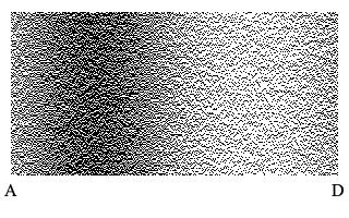
Figure 1: Population of black pixels on a field of white. The relative concentration of black pixels conforms to the probability density function shown in Figure 2.
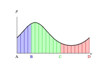
Figure 2: Graph of a continuous probability density function ranging from A to D. The vertical (p)
scale ranges from zero to unity.
The graphic in Figure 1 was generated using the PDF
shown in Figure 2. My program iterated through the x (outer loop) and y
(inner loop) coordinates of the image, choosing the color for the pixel at each (x, y) position. Each
choice was made by generating a decimal number u between A and D, by locating the
x coordinate from the loop iteration along the v axis of
Figure 2 to obtain a density value ρ (ranging from zero to unity), by choosing color
BLACK
when u ≤ ρ, and by choosing color
WHITE otherwise.
Understand that Figure 2 presents a density function, that
density measures concentration per unit, and that when the units drop to zero you
get nothing. Thus the probability that random variable r distributed according to Figure 2
will match any specific v is zero.
To accommodate the nature of density one must think in terms of intervals rather than single points. The probability that r
will lie within a certain interval is then given by the area under the density curve for that particular interval.
Deriving a closed mathematical formula for the area under the curve, even when one already has a formula for the curve itself, often fails.
For example, no closed formula has been successfully derived for the familiar bell curve. However, a curve such as that in Figure 2
can be approximated by trapezoids whose area is easily calculated as base times average height. This is how the
ContinuousDistribution class operates.
Notice in Figure 2 that the range from A to D has been divided into twenty equal-sized intervals. Let vk
indicate the leftmost v coordinate of the kth interval. Then
vk+1 = vk+Δv where Δv = (D−A)/20
is the constant interval width. Also, each interval forms the base of a trapezoidal area with base Δv, with leftmost
height f(vk), and with rightmost height f(vk+1). To
close approximation, the probability that r will fall within the kth interval can
be calculated as the area of the kth trapezoid. (This assumes that the
twenty areas sum to unity, which is the convention for probability density functions.)
The probability that r will fall within any set of intervals in Figure 2 can be calculated as
the sum of the corresponding areas. Thus:
-
Calculating the probability that r will fall between A
and B means adding together the four blue trapezoids (about 0.3).
-
Calculating the probability that r
will fall between B
and C means adding together the eight green trapezoids (about 0.5).
-
Calculating the probability that r will fall between C
and D means adding together the eight pink trapezoids (about 0.2).
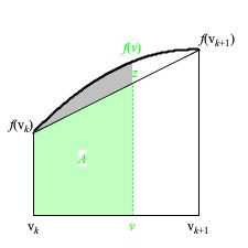
Figure 3: Trapezoidal approximation of function f over the interval from vk to vk+1.
Figure 3 drills down to a single trapezoid, illustrating its features. The base of the trapezoid runs from
vk on the left to vk+1 on the right, giving a width
of Δv.
The thick rising but downward-bending curve plots the values
of function f — understand that this curve has been exaggerated to allow room for the symbol z.
The sloped line running from f(vk) through z to
f(vk+1) is called the line of interpolation.
The symbol z itself indicates the approximation to f at
distribution-range value v.
The vertical distance from f(vk) to f(vk+1)
will henceforth be indicated as Δp. This will allow us to indicate the
slope of the interpolation line as Δp/Δv.
Approximating the probability density f(v) for the distribution-range value
v involves first identifying which range interval encloses v;
this first step establishes f(vk) as a coarse approximation for z.
The second step uses the slope Δp/Δv to refine the approximation. It locates
z along the line of interpolation by determining how far up or down
z will move as v
progresses rightward from vk.
This calculation is known as linear interpolation:
An alternative approach which I favor expresses the distance from vk to
v as a proportion relative to the distance Δv
from vk to vk+1:
u = (v−vk) / (vk+1−vk) = (v−vk) / Δv
The intermediate variable u is called an interpolation factor.
It abstracts the v axis out of the calculation, leaving just a vertical (probability domain) coordinate
f(vk) and a vertical distance Δp :
z = f(vk) + u(f(vk+1)−f(vk)) = f(vk) + uΔp
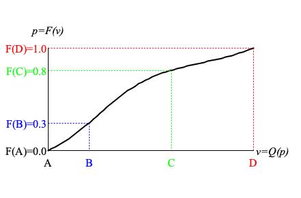
Figure 4: Graph of a cumulative distribution function derived from the continuous densities graphed in Figure 2. The horizontal (v) scale is
the distribution range from A to D. The vertical (p) scale extends from zero (certain not to occur) to unity (certain to occur).
The CDF for a continuous distribution
maps values from the range to always-expanding portions of the probability domain; each
portion indicating how many sample values are < the function argument.
As Figure 4 illustrates, the CDF with the range on the horizontal axis
presents visually as an always-ascending curve:
-
F(A)=0.0 indicates that no sample values are < A.
-
From A to B, the CDF increases
fairly steeply while bending upward. This happens because the PDF in Figure 2
peaks just after B.
-
F(B)=0.3 indicates that 30% of samples have values between A and B.
-
From B to C, the CDF in Figure 4 also increases
fairly steeply but now with a downward bend. Here the PDF mostly recedes from its peak.
-
F(C)=0.8 indicates that 80% of samples have values between A and C.
-
From C to D, the CDF in Figure 4 increases
more gradually owing to the trough in the PDF about 3/8 of the distance from C to D.
The CDF bends downward as the PDF recedes into the trough, then bends upward once the
trough has been attained.
-
F(D)=1.0 indicates that the entire population of samples has values between A and D.
Referring back to Figure 3, notice the light-green shaded area marked A along with
the gray-shaded area above the line of interpolation.
These shaded areas together represent the true area under the f curve from
vk to v.
The light-green shaded area A by itself approximates the true area only to the extent
that the line of interpolation conforms to f. The gray-shaded area indicates the error associated
with the approximation, which can typically be reduced by decreasing Δv.
Approximating the CDF for the distribution-range value
v begins by identifying which range interval encloses v.
Suppose v is enclosed by the kth
range interval. The approximated CDF — F*(vk) — becomes a
coarse approximation which can then be refined by determining how much
A will increase from zero as
v progresses rightward from vk.
A will never decrease because probability densities may never be negative.
The area A has base (v−vk) and average height
(f(vk)+z)/2, where
z approximates the PDF at
v. Calculating area as base × average height gives:
Therefore,
F*(v) = F*(vk) + (v−vk)×(f(vk)+z)/2
It might seem intimidating that F*(vk)
is the sum of all trapezoidal areas left of the current distribution-range interval. However, all of these trapezoidal
areas are known at construction time. Each F*(vk)
can therefore be precalculated and stored as part of the construction process.
The quantile function for a continuous distribution
maps specific values from the probability domain to specific range
values. The quantile function is the mathematical inverse of the CDF, meaning that
if p = F(v) in Figure 4 then
v = Q(p).
Thus the quantile graph
is the same as the CDF graph, just used differently. The probability-domain (p) axis plots the independent
input, while the range (v) axis plots the dependent output.
Let p be a probability-domain amount ranging from zero to unity.
Approximating the quantile-function value at p begins by identifying the range interval for which
F*(vk)
is ≤ p and for which
F*(vk)+A(vk+1) is > p.
The distribution-range value vk becomes a coarse approximation which can then be refined by treating
p−CDF(vk) as an area under the interpolation
line, then determing what v must be to achieve that area.
Expressed using the symbols of Figure 3, the above discussion of CDF stated:
A = (v−vk) × (f(vk)+z)/2
The earlier discussion of PDF stated that z is
interpolated between f(vk)
and f(vk+1):
z = f(vk) + (Δp/Δv)×(v−vk)
Substituting this z into the equation for A gives:
A = (v−vk) × (f(vk) + f(vk) + (Δp/Δv)×(v−vk))/2
Recombining terms to form a quadratic equation gives:
(Δp/Δv)×(v−vk)2 + 2×f(vk)×(v−vk) − 2×A = 0
Applying the quadratic formula gives:
This is the quantile function for a trapezoidal distribution whose probability densities change linearly from f(vk)
to f(vk+1).
Only the positive square root is relevant, since (v-vk) cannot be negative.
To validate this result, first suppose A = 0. Then
Now suppose A = Δv × (f(vk)+f(vk+1))/2 = Δv × (f(vk)+(Δp/2)). Then
| (v−vk) |
= |
| -f(vk) + √f(vk)2 + 2×(Δp/Δv)×Δv×(f(vk)+(Δp/2)) |
| Δp/Δv |
|
|
= |
| -f(vk) + √f(vk)2 + 2×Δp ×(f(vk)+(Δp/2)) |
| Δp/Δv |
|
|
= |
| -f(vk) + √f(vk)2 + 2×Δp ×f(vk)+×Δp 2 |
| Δp/Δv |
|
|
= |
| -f(vk) + f(vk) + Δp |
| Δp/Δv |
|
|
= |
Δv |
/**
 * The {@link ContinuousDistribution} class maps double-precision values
 * to densities.
 * It approximates a smooth distribution curve using a sequence of trapezoidal
 * approximations.
 * @author Charles Ames
 */
public class ContinuousDistribution
extends DistributionBase<Double> {

   private static ContinuousDistribution normalDistribution = null;
   private ContinuousDistributionContour contour;
   private double numericalMean;
   private double numericalVariance;
   private double sumOfWeights;
   private double minOrdinate;
   private double maxOrdinate;
   /**
    * Constructor for {@link ContinuousDistribution} instances
    * @param container A {@link WriteableEntity} which contains this
    * distribution.
    */
   public ContinuousDistribution(WriteableEntity container) {
      super(container);
      this.contour = new ContinuousDistributionContour(this);
      this.contour.setDefaultValue(0.);
      initialize();
   }
   /**
    * Constructor for {@link ContinuousDistribution} instances
    * @param container A {@link WriteableEntity} which contains this
    * distribution.
    * @param name The unit name, which must be unique under the
    * container.
    */
   public ContinuousDistribution(WriteableEntity container, String name) {
      this(container);
      setName(name);
   }
   public void initialize() {
      this.numericalMean = Double.NaN;
      this.numericalVariance = Double.NaN;
      this.sumOfWeights = Double.NaN;
      contour.clearSegments();
   }
   /**
    * Add a region from which this distribution can select a value.
    * @param left The lower bound of the region.
    * @param right The upper bound of the region.
    * @param origin The density for values near the lower bound.
    * @param goal The density for values near the upper bound.
    * @return The newly created region.
    * @throws UnsupportedOperationException when the distribution
    * has already been normalized.
    */
   public ContinuousDistributionItem addItem(
         double left, double right, Double origin, Double goal) {
      if (isNormalized())
         throw new UnsupportedOperationException(
               "Distribution has already been normalized");
      ContinuousDistributionItem item
         = (ContinuousDistributionItem) contour.createSegment(left, right, origin, goal);
      return item;
   }
   /**
    * Get the item with the heaviest weight.
    * @return The value component with the heaviest weight.
    */
   public ContinuousDistributionItem heaviestItem() {
      if (!isNormalized())
         throw new UnsupportedOperationException(
               "Distribution has not been normalized");
      double peakWeight = 0.;
      ContinuousDistributionItem result = null;
      Iterator<Segment<Double, Double>> iterator
         = contour.iterateSegments();
      while (iterator.hasNext()) {
         ContinuousDistributionItem item
            = (ContinuousDistributionItem) iterator.next();
         double weight = item.getArea();
         if (weight > peakWeight) {
            result = item;
            peakWeight = weight;
         }
      }
      if (null == result)
         throw new RuntimeException("No peak value found");
      return result;
   }
   /**
    * Iterate through this distribution's items.
    * @return An iterator of contour segments, each of which
    * can be cast to a {@link ContinuousDistributionItem}.
    */
   public Iterator<Segment<Double, Double>> iterateSegments() {
      return contour.iterateSegments();
   }
   @Override
   public void normalize() {
      sumOfWeights = 0.;
      numericalMean = 0.;
      minOrdinate = ContourFromReal.MAX_ORDINATE;
      maxOrdinate = ContourFromReal.MIN_ORDINATE;
      Iterator<Segment<Double, Double>> iterator
         = contour.iterateSegments();
      int index = 0;
      double total = 0.;
      while (iterator.hasNext()) {
         ContinuousDistributionItem item
            = (ContinuousDistributionItem) iterator.next();
         Double left = item.getLeft();
         Double right = item.getRight();
         Double weight;
         if (0 == index)  {
            weight = item.getOrigin();
            numericalMean += left * weight;
            total += weight;
         }
         weight = item.getGoal();
         numericalMean += right * weight;
         total += weight;
         weight = item.getArea();
         item.setSum(sumOfWeights);
         sumOfWeights += weight;
         minOrdinate = Math.min(minOrdinate, left);
         maxOrdinate = Math.max(maxOrdinate, right);
         index++;
      }
      numericalMean /= total;
      numericalVariance = 0.;
      iterator = contour.iterateSegments();
      index = 0;
      while (iterator.hasNext()) {
         ContinuousDistributionItem item
            = (ContinuousDistributionItem) iterator.next();
         double d;
         if (0 == index)  {
            d = item.getLeft() - numericalMean;
            numericalVariance += item.getOrigin() * d * d;
         }
         d = item.getRight() - numericalMean;
         numericalVariance += item.getGoal() * d * d;
         index++;
      }
      numericalVariance /= total;
   }
   @Override
   public boolean isNormalized() {
      return sumOfWeights > 0.;
   }
   private ContinuousDistributionItem locateItem(Double value) {
      ContinuousDistributionItem item
         = (ContinuousDistributionItem) contour.locateSegment(value);
      if (null == item) {
         System.out.println(contour.dumpSegments());
         throw new IllegalArgumentException(
            "Invalid argument " + MathMethods.formatDouble(value, 3));
      }
      return item;
   }
   private ContinuousDistributionItem chooseItem(
         double chooser, int low, int high) {
      if (low > high)
         throw new RuntimeException(
               "Cannot locate segment for driver value "
               + (chooser / sumOfWeights()));
      int mid = (low + high) / 2;
      ContinuousDistributionItem item = getItem(mid);
      double lowerSum = item.getSum();
      if (chooser < lowerSum) return chooseItem(chooser, low, mid-1);
      double upperSum = lowerSum + item.getArea();
      if (chooser >= upperSum) return chooseItem(chooser, mid+1, high);
      return item;
   }
   @Override
   public Double minRange() {
      return getItem(0).getLeft();
   }
   @Override
   public Double maxRange() {
      return getItem(itemCount()-1).getRight();
   }
   /**
    * Get the distance from the lower range boundary to the upper range boundary.
    * @return The difference between distribution range boundaries.
    */
   public Double spanRange() {
      return maxRange() - minRange();
   }
   @Override
   public Double maxGraphValue(double tail) {
      DistributionBase.checkTail(tail);
      if (!isNormalized())
         throw new IllegalArgumentException(
            "Distribution has not been normalized");
      double threshold = (1. - tail) * sumOfWeights();
      for (int index = itemCount(); --index >= 0;) {
         ContinuousDistributionItem item = getItem(index);
         if (item.getSum() + item.getArea() < threshold) {
            return item.getRight();
         }
      }
      throw new RuntimeException("No maximum graph value");
   }
   @Override
   public Double minGraphValue(double tail) {
      DistributionBase.checkTail(tail);
      if (!isNormalized())
         throw new IllegalArgumentException(
            "Distribution has not been normalized");
      double threshold = sumOfWeights() * tail;
      for (int index = 0; index < itemCount(); index++) {
         ContinuousDistributionItem item = getItem(index);
         if (item.getSum() + item.getArea() > threshold) {
            return item.getLeft();
         }
      }
      throw new RuntimeException("No maximum graph value");
   }
   @Override
   public double densityAt(Double value) {
      return contour.valueAt(value) / sumOfWeights();
   }
   @Override
   public double densityUpTo(Double value) {
      ContinuousDistributionItem item = locateItem(value);
      return (item.getSum()+item.areaUpTo(value))/sumOfWeights();
   }
   /**
    * Divide the range of this distribution into equal-width regions
    * and sum up the probability density in each region.
    * @param regionCount The number of regions.
    * @return A {@link java.util.List} of newly created
    * {@link ContinuousDistributionRegion} instances, which together span
    * the range of the distribution.
    */
   public List<ContinuousDistributionRegion> calculateRegions(int regionCount) {
      List<ContinuousDistributionRegion> regions
         = new ArrayList<ContinuousDistributionRegion>();
      double minRange = minRange();
      double maxRange = maxRange();
      double regionWidth = (maxRange - minRange) / regionCount;
      double left = minRange;
      double sum = 0.;
      for (int regionIndex = 0; regionIndex < regionCount; regionIndex++) {
         double right = Math.min(left + regionWidth, maxRange);
         double current = densityUpTo(right);
         double weight = current - sum;
         ContinuousDistributionRegion region
            = new ContinuousDistributionRegion(left, right, weight);
         regions.add(region);
         sum = current;
         left = right;
      }
      if (!MathMethods.haveSmallDifference(sum, 1.))
         throw new RuntimeException(
            "Regions sum to " + MathMethods.formatDouble(sum, 3) + " which is not unity");
      return regions;
   }
   @Override
   public double maxDensity() {
      ContinuousDistributionItem item = heaviestItem();
      return item.getArea() / item.getWidth() / sumOfWeights();
   }
   @Override
   public double sumOfWeights() {
      if (!isNormalized())
         throw new RuntimeException(
            "Sum of values may not be accessed until distribution has been normalized");
      int itemCount = itemCount();
      if (0 == itemCount)
         throw new RuntimeException("No distribution items");
      return sumOfWeights;
   }
   @Override
   public int itemCount() {
      return contour.segmentCount();
   }
   /**
    * Dereference a (region, weight) element from the collection.
    * @param index The position of the desired element.
    * @return The desired element.
    * @throws IndexOutOfBoundsException when the index is out of range.
    */
   public ContinuousDistributionItem getItem(int index) {
      return (ContinuousDistributionItem) contour.segmentAt(index);
   }
   /**
    * Use the indicated driver to select a value.
    * The selection process first multiplies the driver by the sum of
    * region weights to derive a "chooser" variable. The process then steps
    * through the collection of regions, comparing chooser to weight.  If
    * the chooser is less than or equal to the region weight, then the
    * current region is selected.  Otherwise, the current weight is
    * subtracted from the chooser, and the next region is considered.
    * Once a region has been selected, then the residual chooser places
    * the value within the region. Residuals tending toward zero yield values
    * tending toward the lower region boundary.  Residuals tending toward the
    * region weight yield values tending toward the upper region boundary.
    * @param driver The indicated driver.
    * @return The selected value.
    * @throws IllegalArgumentException when the driver value falls outside
    * the range from zero to unity.
    */
   public Double quantile(double driver) {
      if (!isNormalized())
         throw new IllegalArgumentException("Distribution has not been normalized");
      double chooser = driver * sumOfWeights();
      ContinuousDistributionItem item = chooseItem(chooser, 0, itemCount() - 1);
      double result = item.chooseValue(chooser);
      if (result < minOrdinate || result > maxOrdinate) {
         throw new RuntimeException(
            "Result [" + result + " outside range from "
            + minOrdinate + " to " + maxOrdinate);
      }
      return result;
   }
   /**
    * Generate a distribution to produce an equal-ratios
    * contour from the origin weight as of leftmost value (zero) to
    * the goal weight as of the rightmost value (unity).
    * @param origin The weight as of the leftmost range value (zero).
    * @param goal The weight as of the rightmost range value (unity).
    * @param itemCount The number of trapezoidal regions.
    * @throws IllegalArgumentException when the origin is not positive.
    * @throws IllegalArgumentException when the goal is not positive.
    * @throws IllegalArgumentException when the item count is fewer than 8.
    */
   public void calculateProportional(double origin, double goal, int itemCount) {
      if (MathMethods.TINY > origin)
         throw new IllegalArgumentException("Origin must be positive");
      if (MathMethods.TINY > goal)
         throw new IllegalArgumentException("Goal must be positive");
      if (8 > itemCount)
         throw new IllegalArgumentException("Item count must be 8 or larger");
      initialize();
      if (MathMethods.haveSmallDifference(origin, goal)) {
         addItem(0., 1., origin, goal);
      }
      else {
         double y = origin;
         double x = 0.;
         double increment = 1. / itemCount;
         while (x < 1.) {
            double nextX = x + increment;
            double nextY = calcProportional(nextX, origin, goal);
            addItem(x, nextX, y, nextY);
            x = nextX;
            y = nextY;
         }
      }
      normalize();
   }
   private double calcProportional(double x, double origin, double goal) {
      if (goal > origin) {
         return origin * Math.pow(goal/origin, x);
      }
      return goal * Math.pow(origin/goal, 1.-x);
   }
   /**
    * Generate a one region distribution to produce a straight-line
    * contour from the origin weight as of leftmost value zero to
    * the goal weight as of the rightmost value unity.
    * @param origin The weight as of the leftmost range value (zero).
    * @param goal The weight as of the rightmost range value (unity).
    * @throws IllegalArgumentException when the origin is negative.
    * @throws IllegalArgumentException when the goal is negative.
    * @throws IllegalArgumentException when both the origin and the goal
    * are zero.
    */
   public void calculateTrapezoidal(double origin, double goal) {
      initialize();
      addItem(0., 1., origin, goal);
      normalize();
   }
   /**
    * Generate regions for this distribution to produce a standard
    * bell-curve with the indicated mean, deviation, extent, and grain.
    * The standard bell curve is also known as the Normal distribution
    * or the Gaussian distribution.
    * It was actually first developed by Abraham DeMoivre.
    * @param mean The mid-point of the bell curve.
    * @param deviation The spread of the bell curve around its mid-point.
    * @param extent The distance from lowest range value to highest range
    * value, in standard deviations.
    * @param itemCount The number of trapezoidal regions.
    * @throws IllegalArgumentException when the deviation is not positive.
    * @throws IllegalArgumentException when the extent is not positive.
    * @throws IllegalArgumentException when the item count is less than 8.
    */
   public void calculateNormal(
         double mean, double deviation, double extent, int itemCount) {
      if (MathMethods.TINY > deviation)
         throw new IllegalArgumentException("Deviation must be positive");
      if (2. > extent)
         throw new IllegalArgumentException("Extent must exceed two standard deviations.");
      if (8 > itemCount) throw new IllegalArgumentException("Item count must be 8 or larger");
      initialize();
      double z = -1. / (2.*deviation*deviation);
      double x = mean - (0.5 * extent * deviation);
      double increment = extent * deviation / itemCount;
      double y = calcNormal(x, mean, z);
      for (int index = 0; index < itemCount; index++) {
         double nextX = x + increment;
         double nextY = calcNormal(nextX, mean, z);
         addItem(x, nextX, y, nextY);
         x = nextX;
         y = nextY;
      }
      normalize();
   }
   private double calcNormal(double x, double mean, double z) {
      double d = x - mean;
      return Math.exp(d*d*z);
   }
   /**
    * Method for generating a member of a two-parameter
    * exponential family of curves with the indicated alpha, beta, extent, and grain.
    * A chi-square distribution happens when alpha is r/2 and beta is 2.
    * A negative exponential distribution happens when alpha is 1 and beta is 1/lambda.
    * @param shape The shape parameter.
    * @param scale The scale parameter.
    * @param extent The distance from lowest range value to highest range
    * value, in standard deviations.
    * @param itemCount The number of trapezoidal regions.
    * @throws IllegalArgumentException when the alpha parameter is not positive.
    * @throws IllegalArgumentException when the beta parameter is not positive.
    * @throws IllegalArgumentException when the extent is not positive.
    * @throws IllegalArgumentException when the item count is less than 8.
    */
   public void calculateGamma(
         double shape, double scale, double extent, int itemCount) {
      if (MathMethods.TINY > shape)
         throw new IllegalArgumentException("Alpha must be positive");
      if (MathMethods.TINY > scale)
         throw new IllegalArgumentException("Beta must be positive");
      if (2. > extent)
         throw new IllegalArgumentException("Extent must exceed two standard deviations");
      if (8 > itemCount)
         throw new IllegalArgumentException("Item count must be 8 or larger");
      initialize();
      double mean = shape * scale;
      double deviation = Math.sqrt(mean * scale);
      double maxVal = extent * deviation;
      double x = 0.;
      double increment = maxVal / itemCount;
      double y = calcGamma(x, shape, scale);
      for (int index = 0; index < itemCount; index++) {
         double nextX = x + increment;
         double nextY = calcGamma(nextX, shape, scale);
         addItem(x, nextX, y, nextY);
         x = nextX;
         y = nextY;
      }
      normalize();
   }
   private double calcGamma(double x, double shape, double scale) {
      return Math.pow(x, shape-1)*Math.exp(-x/scale);
   }
   /**
    * Method for generating John Myhill's generalization of the negative
    * exponential distribution.
    * @param scale The scale parameter.
    * @param ratio The ratio of largest range value lowest range
    * value.
    * @param itemCount The number of trapezoidal regions.
    * @throws IllegalArgumentException when the scale parameter is not positive.
    * @throws IllegalArgumentException when the ratio parameter is not greater than unity.
    * @throws IllegalArgumentException when the item count is less than 8.
    */
   public void calculateMyhill(double scale, double ratio, int itemCount) {
      if (MathMethods.TINY > scale)
         throw new IllegalArgumentException("Scale must be positive");
      if (MathMethods.ONE_PLUS > ratio)
         throw new IllegalArgumentException("Ratio must be greater than unity");
      if (8 > itemCount)
         throw new IllegalArgumentException("Item count must be 8 or larger");
      double u2 = Math.pow(ratio, 1. / (1. - ratio));
      double u1 = Math.pow(u2, ratio);
      double low = -scale * Math.log(u2);
      double high = -scale * Math.log(u1);
      initialize();
      double span = high - low;
      double increment = span / itemCount;
      double x = low;
      double y = calcMyhill(x, scale);
      for (int index = 0; index < itemCount; index++) {
         double nextX = x + increment;
         double nextY = calcMyhill(nextX, scale);
         addItem(x, nextX, y, nextY);
         x = nextX;
         y = nextY;
      }
      normalize();
   }
   private double calcMyhill(double x, double scale) {
      return Math.exp(-x*scale);
   }
   /**
    * Method for generating a member of a two-parameter
    * beta family of curves with the indicated alpha, beta, and grain.
    * A continuous uniform distribution happens when alpha is 1 and beta is 1.
    * @param alpha Left-side emphasis.
    * @param beta Right-side emphasis.
    * @param itemCount The number of trapezoidal regions.
    * @throws IllegalArgumentException when the alpha parameter is not positive.
    * @throws IllegalArgumentException when the beta parameter is not positive.
    * @throws IllegalArgumentException when the item count is less than 8.
    */
   public void calculateBeta(double alpha, double beta, int itemCount) {
      if (MathMethods.TINY > alpha)
         throw new IllegalArgumentException("Alpha must be positive");
      if (MathMethods.TINY > beta)
         throw new IllegalArgumentException("Beta must be positive");
      if (8 > itemCount)
         throw new IllegalArgumentException("Item count must be 8 or larger");
      initialize();
      double x = 0.;
      double increment = 1. / itemCount;
      double y = calcBeta(x, alpha, beta);
      for (int index = 0; index < itemCount; index++) {
         double nextX = x + increment;
         double nextY = calcBeta(nextX, alpha, beta);
         addItem(x, nextX, y, nextY);
         x = nextX;
         y = nextY;
      }
      normalize();
   }
   private double calcBeta(double x, double alpha, double beta) {
      return Math.pow(x, alpha-1.)*Math.pow(1.-x, beta-1.);
   }
   /**
    * Method for generating probability curve where the range from zero to one
    * is one turn around a circle and weights go from sqrt(ratio) when
    * x is 0 (0 degrees) to 1 when x is 0.25 (90 degrees) to sqrt(1/ratio) when
    * x is 0.5 (180 degrees) to 1 when x is 0.75 and back to ratio when x
    * is 1.0 (360 degrees).
    * @param turns The ratio of the maximum weight to minimum weight.
    * @param ratio The ratio of the maximum weight to minimum weight.
    * @param itemCount The number of trapezoidal regions.
    * @throws IllegalArgumentException when the ratio parameter is less than unity.
    * @throws IllegalArgumentException when the item count is less than 8.
    */
   public void calculateCosexp(double turns, double ratio, int itemCount) {
      if (0. > turns || 1. < turns)
         throw new IllegalArgumentException("Turns must be between zero and unity");
      if (1. > ratio)
         throw new IllegalArgumentException("Ratio must be at least 1");
      if (8 > itemCount)
         throw new IllegalArgumentException("Item count must be 8 or larger");
      initialize();
      double x = 0.;
      double increment = 1. / itemCount;
      double base = Math.sqrt(ratio);
      double y = calcCosexp(x - turns, base);
      for (int index = 0; index < itemCount; index++) {
         double nextX = x + increment;
         double nextY = calcCosexp(nextX - turns, base);
         addItem(x, nextX, y, nextY);
         x = nextX;
         y = nextY;
      }
      normalize();
   }
   private double calcCosexp(double value, double base) {
      double radians = MathMethods.radiansFromTurns(value);
      return Math.pow(base, Math.cos(radians));
   }
   /**
    * Get a normal distribution centered around zero with deviation one.
    * @return A {@link ContinuousDistribution} instance
    */
   public static ContinuousDistribution getNormalDistribution() {
      if (null == normalDistribution) {
         normalDistribution = new ContinuousDistribution(null);
         normalDistribution.calculateNormal(0, 1, 12, 200);
      }
      return normalDistribution;
   }
   @Override
   public double numericalMean() {
      if (!isNormalized())
         throw new IllegalArgumentException(
            "Distribution has not been normalized");
      return numericalMean;
   }
   @Override
   public double numericalVariance() {
      if (!isNormalized())
         throw new IllegalArgumentException(
            "Distribution has not been normalized");
      return numericalVariance;
   }
}
Listing 1: The
ContinuousDistribution implementation class.
/**
 * Refinement of {@link RealContourFromReal} which uses
 * {@link net.charlesames.utility.contour.Contour.CalculationMode#LINEAR} interpolation and permits no
 * negative abscissas.
 * @author Charles Ames
 */
public class ContinuousDistributionContour extends RealContourFromReal {
   /**
    * Constructor for {@link ContinuousDistributionContour} instances with container.
    * @param container The entity that contains this contour (may be null).
    */
   public ContinuousDistributionContour(WriteableEntity container) {
      super(container);
      this.setIDQuality(AttributeQuality.UNUSED);
      this.setNameQuality(AttributeQuality.UNUSED);
      this.setCalculationMode(CalculationMode.LINEAR);
   }
   @Override
   protected ContinuousDistributionItem newSegment(Double left,
         Double right, Double origin, Double goal) {
      if (origin < 0. && origin > -MathMethods.TINY) origin = 0.;
      if (goal < 0. && goal > -MathMethods.TINY) goal = 0.;
      return new ContinuousDistributionItem(this, left, right, origin, goal);
   }
}
Listing 2: The
ContinuousDistributionContour implementation class.
/**
 * The {@link ContinuousDistributionItem} class defines a region of a
 * continuous distribution and the densities associated with this region.
 * @author Charles Ames
 */
public class ContinuousDistributionItem extends RealSegmentFromReal {
   private double area;
   private double sum;
   private double valueSum;
   private double originSquared;
   private double deltaValue;
   private double deltaDensity;
   private double slope;
   protected ContinuousDistributionItem(ContourFromReal<Double> contour,
         double left, double right, double origin, double goal) {
      super(contour, left, right, origin, goal);
      if (origin < 0.)
         throw new IllegalArgumentException(
            "Origin is negative");
      if (goal < 0.)
         throw new IllegalArgumentException
         ("Goal is negative");
      calculateArea();
      this.sum = Double.NaN;
   }
   private void calculateArea() {
      valueSum = getOrigin() + getGoal();
      deltaDensity = getGoal() - getOrigin();
      deltaValue = getRight() - getLeft();
      slope = deltaDensity / deltaValue;
      originSquared = getOrigin()*getOrigin();
      area = (valueSum * deltaValue) / 2.;
   }
   protected boolean setOrigin(Double origin) {
      if (origin < -MathMethods.TINY)
         throw new IllegalArgumentException(
            "Origin " + MathMethods.formatDouble(origin, 3) + " is negative");
      if (origin < 0.) {
         return super.setOrigin(0.);
      }
      else {
         return super.setOrigin(origin);
      }
   }
   protected boolean setGoal(Double goal) {
      if (goal < -MathMethods.TINY)
         throw new IllegalArgumentException(
            "Goal " + MathMethods.formatDouble(goal, 3) + " is negative");
      if (goal < 0.) {
         return super.setGoal(0.);
      }
      else {
         return super.setGoal(goal);
      }
   }
   /**
    * Get the area (base times average height) of the region whose
    * base extends from the left range bound to the indicated value.
    * @param value The indicated value.
    * @return The area under the curve from left to value.
    */
   public double areaUpTo(Double value) {
      double height = 0.5 * (getOrigin() + valueAt(value));
      double width = value - getLeft();
      return width * height;
   }
   /**
    * Get the area (base times average height) of this region.
    * @return The area (base times average height) of this region.
    */
   public double getArea() {
      return area;
   }
   /**
    * Get the cumulative area for this region, which is the area of this
    * region plus the cumulative area of the previous region.
    * @return The cumulative area for this region.
    */
   public double getSum() {
      if (Double.isNaN(sum))
         throw new UninitializedException("Sum not initialized");
      return sum;
   }
   protected void setSum(double sum) {
      this.sum = sum;
      makeDirty();
   }
   /**
    * Use the indicated chooser to select a value within this region.
    * @param chooser The indicated chooser.
    * @return The selected value.
    * @throws IllegalArgumentException when the chooser falls outside
    * the range from {@link #sum} to {@link #sum}+{@link #area}.
    */
   public double chooseValue(double chooser) {
      double sum = getSum();
      double c = chooser - sum;
      if (c < 0.)
         throw new IllegalArgumentException(
            "Chooser " + MathMethods.textFromDouble(chooser)
            + " short of lower cumulative sum " + MathMethods.textFromDouble(sum));
      double area = getArea();
      if (c > area) {
         throw new IllegalArgumentException(
            "Chooser " + MathMethods.textFromDouble(chooser)
            + " exceeds upper cumulative sum " + MathMethods.textFromDouble(sum+area));
      }
      double result;
      result = (-getOrigin() + Math.sqrt(originSquared + (2*slope*(c))))
            / slope;
      return getLeft() + result;
   }
}
Listing 3: The
ContinuousDistributionItem implementation class.
There are two continuous distribution classes which together implement a composite design pattern:
A single parent ContinuousDistribution instance (Listing 1) stands for the
whole, while multiple child ContinuousDistributionItem instances (Listing 3) detail the parts.
Package consumers typically interact with the parent only.
The type hierarchy for ContinuousDistribution is:
The type hierarchy for ContinuousDistributionItem is:
The parent ContinuousDistribution class embeds an instance of
ContinuousDistributionContour (in turn extending
RealContourFromReal) to manage the succession of
trapezoids that approximate the probability density function. Notice that
ContinuousDistributionContour.newSegment()
returns ContinuousDistributionItem instances and that
ContinuousDistributionItem ultimately subclasses
from SegmentBase.
(Understand that RealContourFromReal ultimately subclasses
from ContourBase,
the "parent" to SegmentBase's "child".)
Four fields declared by SegmentBase define a trapezoid such as the
one illustrated in Figure 3, which shows an interval of the distribution range
and the interpolation line used to approximate f (the probability density function):
-
The
left field holds the lower bound of the distribution-range interval.
It corresponds to vk in Figure 3.
-
The
right field holds the upper bound of the distribution-range interval,
It corresponds to vk+1 in Figure 3.
-
The
origin field holds the weight as-of left.
It corresponds to f(vk) in Figure 3.
-
The
goal field holds the weight as-of right.
It corresponds to f(vk+1) in Figure 3.
In addition to supporting the PDF with these trapezoidal dimensions,
ContinuousDistributionItem supports the CDF and quantile function with
area and sum fields.
The area fields are calculated upon construction as:
(base)×(average height)
= (right−left)*(origin+goal)/2.
The sum fields are populated by normalize().
For the item in position 0, normalize() sets
sum to 0.
For the item in position k+1, normalize() sets
sum to
sum+area from the item in position k.
I stated above with respect to Figure 2 that probability density
functions conventionally require that the area under the curve, calculated across the entire range, should sum to unity.
However, the implementation of ContinuousDistribution imposes
no such requirement upon its stored contour. Rather, a sumOfWeights
field keeps a running sum of all trapezoidal areas. This running sum is adjusted whenever a new item is added or an existing
item is deleted.
Construction begins with a call to initialize(), next iterates through
calls to addItem(double left, double right, double origin, double goal), and completes with a call to normalize().
The four arguments to addItem() correspond to the four trapezoidal dimensions just listed. Intervals must be presented in ascending
order, and successive intervals must be contiguous. The left argument of the
first addItem() call establishes
the range minimum; the left argument of each successive call must match the right argument of the
previous call; the right argument of the final call establishes the range maximum.
Help in constructing ContinuousDistribution instances is offered by a set of methods for populating
ContinuousDistributionItem instances according to familiar distribution formulas. Each of these
methods starts with a call to initialize(), proceeds with addItem()
calls tailored to the specific distribution formula, and completes with a call to normalize().
All methods have an normalize argument; this determine how many addItem()
calls are made. Methods for distributions which are unbounded either on the right — or in both directions — have an additional
extent argument. The extent determines how far the
distribution's range should extend, measured in standard deviations.
The methods are:
-
calculateProportional(double origin, double goal, int itemCount)
The "proportional" distribution is described on the page devoted to the ContinuousProportional transform.
-
calculateTrapezoidal(double origin, double goal)
The "trapezoidal" distribution employs exactly one ContinuousDistributionItem instance.
It is described on the page devoted to the ContinuousTrapezoidal transform.
-
calculateNormal(double mean, double deviation, double extent, int itemCount)
The normal distribution is described on the page devoted to the
ContinuousNormal transform and also described on the page devoted to the
Brownian driver.
-
calculateGamma(double shape, double scale, double extent, int itemCount)
The gamma distribution is described on the page devoted to the ContinuousGamma transform.
-
calculateMyhill(double scale, double ratio, int itemCount)
The "Myhill" distribution is described on the page devoted to the ContinuousMyhill transform.
-
calculateBeta(double alpha, double beta, int itemCount)
The beta distribution is described on the page devoted to the ContinuousBeta transform.
-
calculateCosexp(double turns, double ratio, int itemCount)
The "cosexp" distribution is described on the page devoted to the ContinuousCosexp transform.
Consumption begins once the call to normalize() returns. The normalize()
method iterates through the ContinuousDistributionItem items, populating each
ContinuousDistributionItem.sum with the CDF up to
— but not including — the current range interval.
Method densityAt(Double value)
implements the PDF. It
leverages RealContourFromReal.valueAt(Double ordinate).
There is some confusing terminology here — the PDF maps range values to probability densities by leveraging a contour which maps
ordinates to values, thus a value for a distribution is an ordinate going in to the contour, while a density for a distribution is a
value coming out of the contour.
Method valueAt() first identifies which ContinuousDistributionItem encloses value
within its left and right boundaries.
(Remember that as far as valueAt() abstracts ContinuousDistributionItem to a
RealSegmentFromReal.)
Having identified the ContinuousDistributionItem, valueAt()
applies the linear interpolation formula derived above to refine the probability density.
This puts things in the situation illustrated in Figure 3, where v corresponds to the
densityAt() method's value
argument, while the return value z is the height of the trapezoid at v.
Since the areas of the distribution's ContinuousDistributionItem instances do not necessarily sum
to unity, it is necessary to divide the result from from valueAt()
by ContinuousDistribution.sumOfWeights.
Method densityUpTo(Double value)
implements the CDF. Like densityAt(),
densityUpTo()
also starts by identifying which ContinuousDistributionItem encloses value.
The CDF at value may then be calculated as the area under the
PDF curve up through left plus the area under the PDF
curve from left to value.
The area up through left is precisely what normalize() populated into
ContinuousDistributionItem.sum.
The area from left to value (actually its close approximation)
appears in Figure 3 as the area shaded light-green. Method
ContinuousDistributionItem.areaUpTo(Double value) implements the partial-area formula derived above.
Method densityUpTo() divides sum+area by
ContinuousDistribution.sumOfWeights, and returns the result.
Method quantile(double driver)
implements the quantile function. It returns an Double range value. Here are the steps:
-
A
double variable chooser is calculated as
driver*sumOfWeights. This happens because
ContinuousDistribution
does not require its trapezoidal areas to sum to unity.
-
Method
chooseItem(double chooser, int low, int high)
implements a binary search to identify which
ContinuousDistributionItem has the
largest sum which is still < chooser.
-
Identifying the item reduces the problem to applying the quantile function for a trapezoidal distribution whose probability densities change linearly from
ContinuousDistributionItem.origin to
ContinuousDistributionItem.goal.
Method chooseValue(double chooser)
applies the above-derived formula to obtain the desired distribution-range value.
| © Charles Ames |
Page created: 2022-08-29 |
Last updated: 2022-08-29 |