Continuous Normal Transform¹

Introduction

The ContinuousNormal transform adapts values from the driver domain to an unbounded range, where the relative concentrations are governed by bell curves centered around the mean sample value.

The range of values output by ContinuousNormal.convert() is symmetric around zero and theoretically unbounded both below and above. A practical upper bound is indirectly controlled by extent, a positive integer maintained as a Java field. The upper bound is calculated by multiplying the extent by the standard deviation.

The shape of the distribution curve is controlled by two parameters: mean, symbolized μ and deviation, symbolized σ, which also controls the scale of the distribution. The mean is not restricted but the deviation must be greater than zero.

ContinuousNormal instances externally reference a shared ContinuousDistribution instance which divides the range from zero to this calculated upper bound into trapezoids of equal width. The number of trapezoids is determined by a fourth parameter maintained as a Java field, itemCount. For the present purposes I have set itemCount to 200.

The trapezoid height for sample value x is calculated using the formula:

For the normal curve, Wikipedia identifies the parametric mean with the mean parameter and the parametric variance with the square of the deviation parameter. The upper bound thus calculates out to:

The practical lower bound minRange is the negative of maxRange. The width of each ContinuousDistribution trapezoid is (maxRange-minRange)/itemCount.

Profile

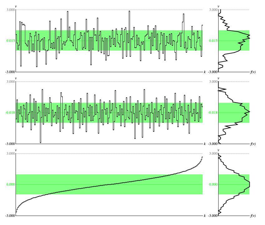
Figure 1 illustrates the influence which ContinuousNormal.convert() exerts over driver sequences when the mean μ = 0 and the deviation σ = 1. This panel was created using the same driver sources used for the ContinuousUniform, which earlier panel provides a basis for comparison.

Figure 1: Panel of ContinuousNormal output from three different Driver sources. Each row of graphs provides a time-series graph of samples (left) and a histogram analyzed from the same samples (right). The first row of graphs was generated using the standard random number generator. The second row was generated using the balanced-bit generator. The third row was generated using an ascending sequence of driver values, equally spaced from zero to unity.

The standard-random time-series graph (top row of Figure 1) has the same relative ups and downs as the standard-random time-series graph prepared for ContinuousUniform, but the specific values are squinched down toward zero. Its hard to see how the driver distribution influences the standard-random histogram presented here, other than the generally ragged shape of the histogram.

The balanced-bit time-series (middle row of Figure 1) likewise has the same ups and downs as the balanced-bit time-series graph prepared for ContinuousUniform with values squinched similarly. Since balanced-bit sequences strive aggressively for uniformity, the jaggedness of this balanced-bit histogram is accodingly moderated.

The time-series graph generated using ascending, equally spaced driver values (bottom row of Figure 1) presents the percentile function for this particular flavor of continuous normal distribution. The histogram of sample values presents the distribution's probability density function or PDF. The PDF is an equal-ratios curve bending upward from f(v) = 1 when v = 0 to f(v) = 3 when v = 1. Looking back at the time-series graph, notice how the ercentile function rises more steeply where the distribution is rarefied and less steeply where the distribution is concentrated.

For each graph in Figure 1 the average sample value is plotted as a dashed green line, while the interval between ± one standard deviation around the average is filled in with a lighter green background. For μ = 0 and σ = 1 the parametric average calculates out to 0, the parametric standard deviation calculates out to 1, and the range extends from -6 to 6. By comparison the numerical average and deviations for the bottom row of graphs were 0.000 and 0.986. Since this bottommost row illustrates the most ideal conditions under which a profile can be generated, these parametric and numerical statistics should match closely, and they do.

The interval from 0.000-0.986 to 0.000+0.986 is 2*0.986 = 1.972. This makes 100*1.972/6 = 33% of the full application range from -6 to 6. Since the continuous uniform distribution had 58% of samples within ± one standard deviation of the mean, this suggests that with the normal distribution with mean 0 and deviation 1 is squeezing 58% of samples into 33% of the application range, giving a concentration rate of 58/33 = 1.76.

The Bell Curve

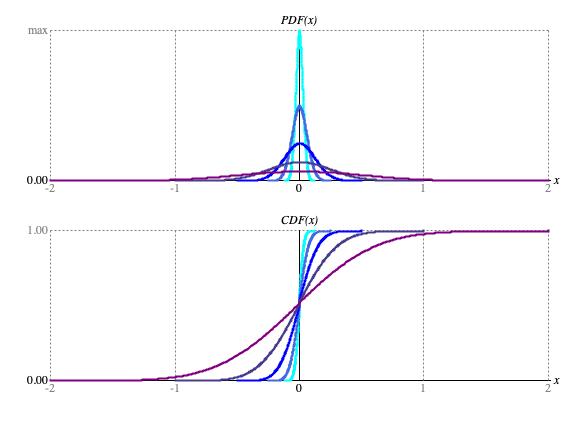
━ σ = 0.03125, ━ σ = 0.06125, ━ σ = 0.125, ━ σ = 0.25, ━ σ = 0.5
Figure 2: Normal distribution curves.

Figures 2 show how changes in deviation settings affect the distribution curves. The figure provides two graphs. The upper graph shows the probability density function or PDF. The lower graph shows the cumulative distribution function or CDF.

/**
 * The {@link ContinuousNormal} class models the standard bell curve over the range from negative infinity to positive infinity.
 * This distribution was devised by Abraham DeMoivre.
 * It is also known as the Normal distribution or the Gaussian distribution.
 * <p>
 * As a statistical transform, {@link ContinuousNormal} does not itself employ probability or randomness.
 * Instead it responds to an externally generated driver sequence which may or may not be random.
 * {@link ContinuousDistribution#quantile(double)} converts the driver value to an outcome.
 * </p>
 * <p>
 * For more information including a graph mapping driver values to results and a second graph showing a random population, see <a href="http://www.jstor.org/stable/1513123"><i>A Catalog of Statistical Distributions</i>, 1991</a>.
 * </p>
 * @author Charles Ames
 */
public class ContinuousNormal
extends TransformBase<Double> implements Transform.Continuous {
   /**
    * Controls the spread of the bell curve around its mid-point.
    */
   private double deviation;
   /**
    * Identifies the mid-point of the bell curve.
    */
   private double mean;
   /**
    * Constructor for {@link ContinuousNormal} instances.
    * @param container An entity which contains this transform.
    */
   public ContinuousNormal(WriteableEntity container) {
      super(container);
      deviation = Double.NaN;
      mean = Double.NaN;
   }
   /**
    * Getter for {@link deviation}.
    * @return The assigned {@link deviation} value.
    */
   public double getDeviation() {
      if (Double.isNaN(deviation)) throw new UninitializedException("Deviation not initialized");
      return deviation;
   }
   /**
    * Setter for {@link deviation}.
    * @param deviation The intended {@link deviation} value.
    */
   public void setDeviation(double deviation) {
      checkDeviation(deviation);
      if (this.deviation != deviation) {
         this.deviation = deviation;
      }
   }
   /**
    * Check if the indicated value is suitable for {@link deviation}.
    * @param deviation The indicated value.
    */
   public void checkDeviation(double deviation) {
      if (deviation < MathMethods.TINY)
         throw new IllegalArgumentException("Deviation not positive");
   }
   /**
    * Getter for {@link mean}.
    * @return The assigned {@link mean} value.
    */
   public double getMean() {
      if (Double.isNaN(mean)) throw new UninitializedException("Mean not initialized");
      return mean;
   }
   /**
    * Setter for {@link mean}.
    * @param mean The intended {@link mean} value.
    */
   public void setMean(double mean) {
      checkMean(mean);
      if (this.mean != mean) {
         this.mean = mean;
      }
   }
   /**
    * Check if the indicated value is appropriate for {@link mean}.
    * @param mean The indicated value.
    */
   public void checkMean(double mean) {
      // No check
   }
   @Override
   public Double minGraphValue(double tail) {
      double value = ContinuousDistribution.getNormalDistribution().minGraphValue(tail);
      return mean + (deviation * value);
   }
   @Override
   public Double maxGraphValue(double tail) {
      double value = ContinuousDistribution.getNormalDistribution().maxGraphValue(tail);
      return mean + (deviation * value);
   }
   @Override
   public Double minRange() {
      return (double) Integer.MIN_VALUE;
   }
   @Override
   public Double maxRange() {
      return (double) Integer.MAX_VALUE;
   }
   @Override
   protected ContinuousDistribution createDistribution() {
      throw new UnsupportedOperationException("Method not implemented");
   }
   @Override
   protected void validate(DistributionBase<Double> distribution) {
      throw new UnsupportedOperationException("Method not implemented");
   }
   @Override
   public Double convert(double driver) {
      Driver.checkDriverValue(driver);
      double value = ContinuousDistribution.getNormalDistribution().quantile(driver);
      value = mean + (deviation * value);
      return value;
   }
}

Comments

1. The present text is adapted from my Leonardo Music Journal article from 1991, "A Catalog of Statistical Distributions". The heading is "Normal", p. 64.