Continuous Myhill Transform¹

Introduction

The ContinuousMyhill transform adapts values from the driver domain to a bounded range, where the relative concentrations are governed by John Myhill's enhancement of the exponential distribution.

John Myhill had his own ideas about how Stochastic Music might be generated by computer programs. At the 1978 ICMC, which Xenakis also attended, Myhill proposed "Some Simplifications and Improvements in the Stochastic Music Program". which presentation initially raised some ire on Xenakis's part. An appendix to this presentation took things a bit farther by advancing a model of "controlled indeterminacy"; in which note timings would transition gradually between pulse rhythms, on one hand, and negative exponential randomness (the timings of successive clicks from a Geiger counter), on the other hand.

The range of values output by ContinuousMyhill.convert() is bounded below by zero and unbounded above.

The shape of the distribution curve is controlled by two parameters: scale, symbolized λ and ratio, symbolized ρ. The scale must be greater than zero and the ratio may not fall below unity. A practical upper bound is indirectly determined by ratio.

Each ContinuousMyhill instance internally maintains a ContinuousDistribution instance which divides the range from zero to this calculated upper bound into trapezoids of equal width. The number of trapezoids is determined by a fourth parameter maintained as a Java field, itemCount. For the present purposes I have set itemCount to 200.

The quantile function mapping a driver argument to an exponentially distributed result exists in closed form, which allows the present implementation to dispense with all the business of trapezoidal approximation in favor of an in-line mathematical expression:

To close things in around the mean, Myhill limited driver values to a subrange from u0 to u1, where 0≤u0<u1≤1. The lower bound u0 is calculated as:

While the upper bound u1 is:

Wikipedia does not recognize the Myhill distribution. The parametric mean (average, symbolized μ) is identical to the scale parameter λ. The variance is 0 when ρ=1 and converges to 1/λ² as ρ increases to infinity.

Profile

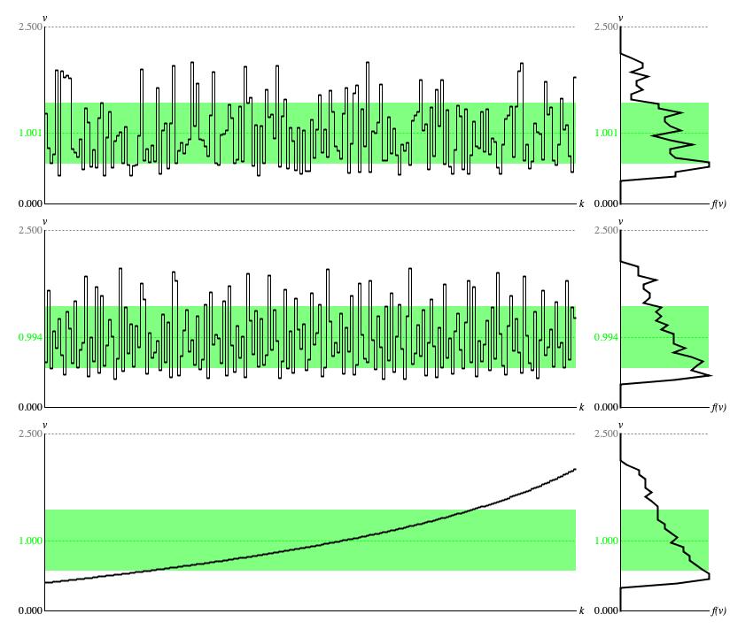
Figure 1 illustrates the influence which ContinuousMyhill.convert() exerts over driver sequences when the scale λ = 1 and the ratio ρ = 5. This panel was created using the same driver sources used for the ContinuousUniform, which earlier panel provides a basis for comparison.

Figure 1: Panel of ContinuousMyhill output from three different Driver sources. Each row of graphs provides a time-series graph of samples (left) and a histogram analyzed from the same samples (right). The first row of graphs was generated using the standard random number generator. The second row was generated using the balanced-bit generator. The third row was generated using an ascending sequence of driver values, equally spaced from zero to unity.

The standard-random time-series graph (top row of Figure 1) has the same relative ups and downs as the standard-random time-series graph prepared for ContinuousUniform, but the specific values are squinched down toward zero. Its hard to see how the driver distribution influences the standard-random histogram presented here, other than the generally ragged shape of the histogram.

The balanced-bit time-series (middle row of Figure 1) likewise has the same ups and downs as the balanced-bit time-series graph prepared for ContinuousUniform with values squinched similarly. Since balanced-bit sequences strive aggressively for uniformity, the jaggedness of this balanced-bit histogram is accodingly moderated.

The time-series graph generated using ascending, equally spaced driver values (bottom row of Figure 1) presents the percentile function for this flavor of Myhill distribution. The histogram of sample values presents the distribution's probability density function or PDF. The PDF is an equal-ratios curve bending upward from f(v) = 1 when v = 0 to f(v) = 3 when v = 1. Looking back at the time-series graph, notice how the percentile function rises more steeply where the distribution is rarefied and less steeply where the distribution is concentrated.

For each graph in Figure 1 the average sample value is plotted as a dashed green line, while the interval between ± one standard deviation around the average is filled in with a lighter green background. For k = 2 and λ = 5 the parametric average calculates out to μ = 2×5 = 10, the parametric standard deviation calculates out to σ = √2×5 = √50 = 7.07, and the upper bound calculates out to 6×7.07 = 42.43. By contrast the numerical average and deviations for the bottom row of graphs were 10.135 and 6.854. Since this bottommost row illustrates the most ideal conditions under which a profile can be generated, these parametric and numerical statistics should match closely. I was able to narrow the gap between parametric and numerical averages by doubling the itemCount, however this change did nothing to close the gap between parametric and numerical deviations. I am hoping that the deviation gap will close with increasing sample counts.

The interval from 10.135-0.280 to 10.135+6.854 is 2*6.854 = 13.708 = 32% of the full application range from zero to unity. Since the continuous uniform distribution had 58% of samples within ± one standard deviation of the mean, this suggests that the Myhill transform with scale 1 and ratio 5 is squeezing 58% of samples into 32% of the application range, giving a concentration rate of 58/32 = 1.81.

The Myhill Probability Curve

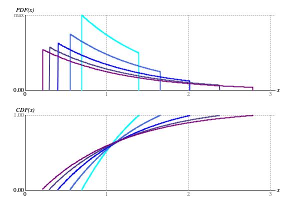
━ ρ = 2, ━ ρ = 3, ━ ρ = 5, ━ ρ = 8, ━ ρ= 13
Figure 2: Myhill distribution curves for shape parameter k = 1.

Figure 2 show how changes in max/min ratios affect the distribution curve. Each figure provides two graphs. The upper graph shows the probability density function or PDF. The lower graph shows the cumulative distribution function or CDF.

When the ratio parameter ρ is large, the Myhill distribution simplifies to the exponential distribution that characterizes waiting durations in the Poisson Point Process.

/**
 * The {@link ContinuousMyhill} class models a continuous distribution devised by John Myhill
 * over the range from zero (exclusive) to infinity.
 * <p>
 * Myhill's distribution extends the negative exponential distribution.
 * The negative exponential distribution models waiting durations between rare events, such as cars passing by on a road
 * (but not during rush hour), or such as beta emissions from a radioactive substance.
 * The one parameter controlling the negative exponential distribution is the mean, or average, duration.
 * </p>
 * <p>
 * John Myhill extended the negative exponential by adding a second parameter to control the ratio between longest to
 * shortest values.  When the ratio is 1, outcomes are strictly periodic.  Durations become increasingly erratic as
 * the ratio increases until
 * </p>
 * <p>
 * As a statistical transform, {@link ContinuousMyhill} does not itself employ probability or randomness.
 * Instead it responds to an externally generated driver sequence which may or may not be random.
 * </p>
 * <p>
 * For more information including a graph mapping driver values to results and a second graph showing a random population, see <a href="http://www.jstor.org/stable/1513123"><i>A Catalog of Statistical Distributions</i>, 1991</a>.
 * </p>
 * @author Charles Ames
 */
public class ContinuousMyhill
extends TransformBase<Double> implements Transform.Continuous {
   /**
    * Controls the proportion between the longest and shortest values.
    */
   private double ratio;
   /**
    * Controls the average value selected (provided that the driving distribution is uniform).
    */
   private double scale;
   private double u1;
   private double u0;
   private boolean valid;
   /**
    * Constructor for {@link ContinuousMyhill} instances.
    * @param container An entity which contains this transform.
    */
   public ContinuousMyhill(WriteableEntity container) {
      super(container);
      ratio = Double.NaN;
      scale = Double.NaN;
      valid = false;
   }
   @Override
   public void wipe() {
      super.wipe();
   }
   /**
    * Getter for {@link #ratio}.
    * @return The assigned {@link #ratio} value.
    * @throws UninitializedException when {@link #ratio} has not been initialized.
    */
   public double getRatio() {
      if (Double.isNaN(ratio)) throw new UninitializedException("Ratio not initialized");
      return ratio;
   }
   /**
    * Setter for {@link #ratio}.
    * @param ratio The intended {@link #ratio} value.
    * @throws IllegalArgumentException when the value is less than unity.
    * @throws IllegalArgumentException when the value exceeds {@link Integer#MAX_VALUE}.
    */
   public void setRatio(double ratio) {
      checkRatio(ratio);
      if (this.ratio != ratio) {
         this.ratio = ratio;
         valid = false;
      }
   }
   /**
    * Check if the indicated value is suitable for {@link #ratio}.
    * @param ratio The indicated value.
    * @throws IllegalArgumentException when the value is less than unity.
    * @throws IllegalArgumentException when the value exceeds {@link Integer#MAX_VALUE}.
    */
   public void checkRatio(double ratio) {
      if (ratio < 1.)
         throw new IllegalArgumentException("Ratio less than unity");
      else if (ratio > Integer.MAX_VALUE)
         throw new IllegalArgumentException("Ratio should not be greater than " + Integer.MAX_VALUE);
   }
   /**
    * Getter for {@link #scale}.
    * @return The assigned {@link #scale} value.
    * @throws UninitializedException when {@link #scale} has not been initialized.
    */
   public double getScale() {
      if (Double.isNaN(scale)) throw new UninitializedException("Scale not initialized");
      return scale;
   }
   /**
    * Setter for {@link #scale}.
    * @param scale The intended {@link #scale} value.
    */
   public void setScale(double scale) {
      checkScale(scale);
      if (this.scale != scale) {
         this.scale = scale;
         valid = true;
      }
   }
   /**
    * Check if the indicated value is suitable for {@link #scale}.
    * @param scale The indicated value.
    * @throws IllegalArgumentException when the value is not positive.
    */
   public void checkScale(double scale) {
      if (scale < MathMethods.TINY)
         throw new IllegalArgumentException("Mean not positive");
   }
   @Override
   public Double minGraphValue(double tail) {
      return 0.;
   }
   @Override
   public Double maxGraphValue(double tail) {
      precalc();
      double z = -scale * Math.log(u1);
      double y = scale * 10;
      if (z > y) z = y;
      return z;
   }
   @Override
   public Double minRange() {
      return 0.;
   }
   @Override
   public Double maxRange() {
      return maxGraphValue(0.);
   }
   @Override
   protected ContinuousDistribution createDistribution() {
      throw new UnsupportedOperationException("Method not implemented");
   }
   @Override
   protected void validate(DistributionBase<Double> distribution) {
      throw new UnsupportedOperationException("Method not implemented");
   }
   public Double convert(double driver) {
      Driver.checkDriverValue(driver);
      precalc();
      double value;
      if (ratio <= MathMethods.ONE_PLUS) {
         value = scale;
      }
      else {
         double arg = (u1 - u0)*driver + u0;
         value = -scale * Math.log(arg);
      }
      return value;
   }
   private void precalc() {
      if (!valid) {
         if (ratio > MathMethods.ONE_PLUS) {
            u0 = Math.pow(ratio, 1. / (1. - ratio));
            u1 = Math.pow(u0, ratio);
         }
         else {
            u0 = Double.NaN;
            u1 = Double.NaN;
         }
         valid = true;
      }
   }
}

Comments

1. The present text is adapted from my Leonardo Music Journal article from 1991, "A Catalog of Statistical Distributions". The heading is "Gamma", p. 65.