Cosine-Exponential Transform¹

Introduction

The ContinuousCosexp transform adapts values from the driver domain to a bounded range which is regarded as one full turn of a circle. The relative concentrations are calculated relative to the .

The range of values output by ContinuousCosexp.convert() is controlled by two parameters implemented as Java fields: minRange and maxRange. These have the restriction that minRange < maxRange. It is strongly recommended that minRange be zero.

The shape of the distribution curve is controlled by two additional parameters: turns (symbolized φ) and ratio (symbolized ρ). The turns parameter is restricted to the range from zero to unity. The ratio parameter must not fall below unity.

Each ContinuousCosexp instance internally maintains a ContinuousDistribution instance which divides the range from zero to unity into trapezoids of width 1/itemCount. The trapezoid height for sample value z is calculated using the formula:

Notice that this formula has a minimum of 1/√ρ when cos(z+turns)=-1 and a maximum of √ρ when cos(z+turns)=1. Therefore the max/min ratio is √ρ/(1/√ρ) = √ρ×√ρ = ρ.

The convert() method maps a value x in the driver domain from zero to unity into a value v in the application-range from minRange to maxRange in two steps. The first step uses ContinuousDistribution.quantile() to recast the driver value x into an intermediate value z, also between zero and unity. The second step applies the linear interpolation formula:

The cosine-exponential distribution was invented by me² — which does not preclude the possibility of it having been invented before by someone unknown to me. Thus Wikipedia supplies neither parametric mean μ nor parametric variance σ² for this distribution.

Profile

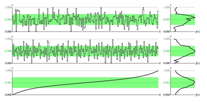
Figure 1 illustrates the influence which ContinuousCosexp.convert() exerts over driver sequences when turns is 0.5 and ratio is 5. This panel was created using the same driver sources used for the ContinuousUniform, which earlier panel provides a basis for comparison.

Figure 1: Panel of ContinuousCosexp output from three different Driver sources. Each row of graphs provides a time-series graph of samples (left) and a histogram analyzed from the same samples (right). The first row of graphs was generated using the standard random number generator. The second row was generated using the balanced-bit generator. The third row was generated using an ascending sequence of driver values, equally spaced from zero to unity.

The standard-random time-series graph (top row of Figure 1) has the same relative ups and downs as the standard-random time-series graph prepared for ContinuousUniform, but the specific values are squinched up toward the upper range bound. This difference becomes much clearer in the standard-random histogram, where the whitespace separating the vertical v axis from the smallest f(v) value progressively increases as v increases from zero to unity. Notice that while these histogram peaks and valleys are similar to those derived for ContinuousUniform, they are not the same. The fact that values squinch upwards means that range values which fell into the bottommost histogram region in the uniform histogram were spread across the bottom three regions here in the cosine-exponential histogram. Likewise the range values which fell into the topmost histogram region here were spread across three regions in the uniform histogram.

The balanced-bit time-series (middle row of Figure 1) likewise has the same ups and downs as the balanced-bit time-series graph prepared for ContinuousUniform with values squinched similarly. Since balanced-bit sequences strive aggressively for uniformity, the histogram peaks and valleys are comparatively restrained.

The time-series graph generated using ascending, equally spaced driver values (bottom row of Figure 1) presents the quantile function for this instance of a cosine-exponential distribution. The histogram of sample values presents the distribution's probability density function or PDF. The PDF is an equal-ratios curve bending upward from f(v) = 1 when v = 0 to f(v) = 3 when v = 1. Looking back at the time-series graph, notice how the quantile function rises more steeply where the distribution is rarefied and less steeply where the distribution is concentrated.

For each graph in Figure 1 the average sample value is plotted as a dashed green line, while the interval between ± one standard deviation around the average is filled in with a lighter green background. For the ideally uniform driver values plotted in the third row of graphs, the average sample value is 0.503 and the standard deviation is 0.217. The interval from 0.719-0.217 to 0.719+0.217 is 2*0.217 = 0.434 = 43% of the full application range from zero to unity. Since the continuous uniform distribution had 58% of samples within ± one standard deviation of the mean, this suggests that with the cosine-exponential distribution with ratio 5 is squeezing 58% of samples into 43% of the application range, giving a concentration rate of 58/43 = 1.35.

Cosine-Exponential Probability Curves

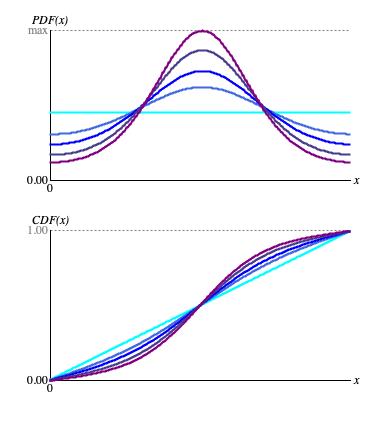
━ ρ = 1, ━ ρ = 2, ━ ρ = 3, ━ ρ = 5, ━ ρ = 8
Figure 2 (a): Cosine-Exponential distribution curves for φ = 0.5 (180°).

Figures 2 (a) through 2 (b) show how changes in parameter settings affect the distribution curves. Each figure provides two graphs. The upper graph shows the probability density function or PDF. The lower graph shows the cumulative distribution function or CDF.

Figure 2 (a) fixes the turns at φ=0.5, centering the peak horizontally over the range. The ratio ranges from ρ=1 (━), which produces no peak at all, through ρ=2 (━), ρ=3 (━), and ρ=5 (━) to ρ=8 (━), where the peak is most prominent.

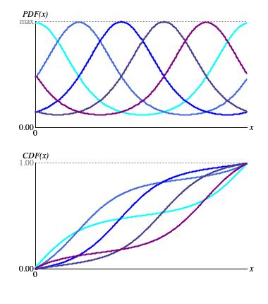
━ φ = 0.0, ━ φ = 0.2, ━ φ = 0.4, ━ φ = 0.6, ━ φ = 0.8
Figure 2 (b): Cosine-Exponential distribution curves for ρ = 8.

Figure 2 (a) fixes the ratio at ρ=8 in order to show how the value of φ positions the peak over the range. Notice that each increment to φ shifts the peak rightward one fifth of the way along the range. Understand that φ=1.0 (not shown) would produce the same graph as φ=0.0.

/**
 * The {@link ContinuousCosexp} class maps driver values back to the range
 * from zero to unity.  Emphasis peaks in center when alpha equals beta; it
 * shifts leftward when alpha < beta and rightward when alpha > beta.  When
 * alpha and beta are both 1, the graph is uniform.
 * @author Charles Ames
 */
public class ContinuousCosexp extends BoundedTransform {
   /**
    * Left-side attenuation.
    */
   private double alpha;
   /**
    * Right-side attenuation.
    */
   private double beta;
   /**
    * Determines the number of trapezoidal regions.
    */
   private int itemCount;
   /**
    * Determines whether a change in parameter values requires the distribution
    * to be recalculated.
    */
   private boolean valid;
   /**
    * Constructor for {@link ContinuousCosexp} instances.
    * @param container An entity which contains this transform.
    */
   public ContinuousCosexp(WriteableEntity container) {
      super(container);
      this.alpha = Double.NaN;
      this.beta = Double.NaN;
      this.itemCount = Integer.MIN_VALUE;
   }
   /**
    * Getter for {@link #alpha}.
    * @return The assigned {@link #alpha} value.
    * @throws UninitializedException when {@link #alpha} has not been initialized.
    */
   public double getAlpha() {
      if (Double.isNaN(alpha)) throw new UninitializedException("Alpha not initialized");
      return alpha;
   }
   /**
    * Setter for {@link #alpha}.
    * Distribution is recalculated.
    * @param alpha The intended {@link #alpha} value.
    * @throws IllegalArgumentException when the argument is not positive.
    */
   public void setAlpha(double alpha) {
      checkAlpha(alpha);
      if (this.alpha != alpha) {
         this.alpha = alpha;
         this.valid = false;
      }
   }
   /**
    * Check if the indicated value is suitable for {@link #alpha}.
    * @param alpha The indicated value.
    * @throws IllegalArgumentException when the argument is not positive.
    */
   public void checkAlpha(double alpha) {
      if (alpha < MathMethods.TINY)
         throw new IllegalArgumentException("Alpha "
               + MathMethods.df3.format(alpha) + " is not positive");
   }
   /**
    * Getter for {@link #beta}.
    * @return The assigned {@link #beta} value.
    * @throws UninitializedException when {@link #beta} is not initialized.
    */
   public double getBeta() {
      if (Double.isNaN(beta))
         throw new UninitializedException("Beta not initialized");
      return beta;
   }
   /**
    * Setter for {@link #beta}.
    * Distribution is recalculated.
    * @param beta The intended {@link #beta} value.
    * @throws IllegalArgumentException when the argument is not positive.
    */
   public void setBeta(double beta) {
      checkBeta(beta);
      if (this.beta != beta) {
         this.beta = beta;
         this.valid = false;
      }
   }
   /**
    * Check if the indicated value is suitable for {@link #beta}.;
    * @param beta The indicated value.
    * @throws IllegalArgumentException when the argument is not positive.
    */
   public void checkBeta(double beta) {
      if (beta < MathMethods.TINY)
         throw new IllegalArgumentException("Beta "
               + MathMethods.df3.format(beta) + " not positive");
   }
   /**
    * Getter for {@link #itemCount}.
    * Distribution is recalculated.
    * @return The assigned {@link #itemCount} value.
    * @throws UninitializedException when {@link itemCount} is not initialized.
    */
   public int itemCount() {
      if (Integer.MIN_VALUE == itemCount)
         throw new UninitializedException("Item count not initialized");
      return itemCount;
   }
   /**
    * Setter for {@link #itemCount}.
    * @param itemCount The intended {@link #itemCount} value.
    */
   public void setItemCount(int itemCount) {
      checkItemCount(itemCount);
      if (this.itemCount != itemCount) {
         this.itemCount = itemCount;
         this.valid = false;
      }
   }
   /**
    * Check if the indicated value is suitable for {@link #itemCount}.
    * @param itemCount The indicated value.
    */
   public void checkItemCount(int itemCount) {
      if (itemCount < 8)
         throw new IllegalArgumentException("Item count too small");
   }
   @Override
   public Double convert(double driver) {
      if (!valid) {
         getDistribution().calculateBeta(getAlpha(), getBeta(), itemCount());
         valid = true;
      }
      return super.convert(driver);
   }
}

Comments

1. The present text is adapted from my Leonardo Music Journal article from 1991, "A Catalog of Statistical Distributions". The heading is "Beta", p. 63
2. A graph appears in my Interface (now Journal of New Music Research) article from 1986, "Two Pieces for Amplified Guitar" p. 39.