Short-Term Uniformity: Balance¹

Introduction

The Balance driver produces sequences which favor short-term uniformity. Samples are assembled bit by bit using statistical feedback.² The decision of whether a certain bit should be set to 1 or cleared to 0 is guided by a statistic s. This statistic keeps track of how often the set state has been used, as opposed to how often the clear state has been used:

• s = 0 indicates that set and clear states have both occured in the same amounts, suggesting that the decision between states should be unbiased.
• s > 0 indicates that set has occured more often than clear, suggesting that the clear state should be favored.
• s < 0 indicates that clear has occured more often than set, suggesting that the set state should be favored.

Just one of these statistics guides bit 1, which determines whether the sample value will fall between 0.0 and 0.5 (bit 1 clear) or between 0.5 and 1.0 (bit 1 set).

Two statistics guide bit 2. One statistic applies when bit 1 is clear; this determines whether the sample value will fall between 0.00 and 0.25 (bit 1 clear, bit 2 clear) or between 0.25 and 0.50 (bit 1 clear, bit 2 set). The other statistic applies when bit 1 is set; this determines whether the sample value will fall between 0.50 and 0.75 (bit 1 set, bit 2 clear) or between 0.75 and 1.00 (bit 1 set, bit 2 set).

Each increment in bit number causes the number of statistics to double. The number of bits affected is controlled by a depth parameter. I usually set this to 6, giving 1+2+4+8+16+32 = 63 statistics for the Balance driver to manage.

Set/clear decisions can be leavened by a heterogeneity parameter, which permits Balance to sometimes make the 'wrong' decision when s is close to zero. Each statistic s reflects the physical usage count for one particular bit under a specific combination of more significant bits. When the heterogeneity is less than one (say 0.1), randomness only exerts influence when s = 0; that is, when the count of set bits equals the count of clear bits. When the heterogeneity setting slightly exceeds one (say, 1.1) then random influence extends to s values -1, 0, and 1. Increasing heterogeneity settings further increase the opportunity to set the bit when it 'ought' to be clear or to clear the bit when it 'ought' to be set. However, s will never range outside ± heterogeneity.

The Balance driver bears a particular relation to Lehmer, which wrap's Java's standard random number generator. Output from both these drivers nominally follows a continuous uniform distribution; however of the two, only Balance realizes this distribution over the short term. In that sense Lehmer is the continuous counterpart of the urn model's selection with replacement, just as Balance is one continuous counterpart of selection without replacement. In this regard, Balance compares to DriverSequence in UsageMode.UNIQUE_SHUFFLE.

Use of either Balance or DriverSequence in place of standard randomness is appropriate when conformity to a distribution trumps the unpredictability of randomness. A good indicator that the distribution is important is the difference between lightest and heaviest distribution weights. Consider a circumstance with ten decisions each having two options. If the options are weighted equally then standard randomness will likely give you five of each, maybe four of one and six of the other, and so forth, with a small but nonzero likelhood of only choosing one option. However suppose option #1 is weighted 9 times more heavily than option #2. With standard randomness it's very likely that option #2 will never appear at all. But by specifying a weight for option #2, you were saying that you wanted option #2 there, just not in quantity. Both Balance and DriverSequence will represent each option fairly. With DriverSequence the presentation won't alternate between options but rather mix them up in an unpredictable order. Balance, by contrast, will present the lightly weighted option quasi-periodically over the extent of the selection cycle.

Now suppose that the weights are evolving over time, that things start out favoring option #1 over option #2 but the weights shift linearly until option #2 has the heavier weight. This situation suggests that occurances of option #2 are initially rare, but that option #2's rate of occurrance gradually increases to the point where option #2 predominates. Neither standard randomness nor shuffling will give you those narrowing occurrance intervals; instead these two approaches will jumble things up. Only balanced-bit selection will pace occurrances according to what rates the weights imply.

The Balance indexer is the continuous counterpart to the Feedback indexer, to the extent that both rely upon statistical feedback. The difference is that Balance produces continuous uniform distributions which must be adapted to non-uniform distributions using an external Transform. Feedback, by contrast, accepts a discrete distribution parametrically.

Profile

Figure 1 illustrates Balance output with sequences of 200 samples generated with depth 6 and various heterogeneity settings.

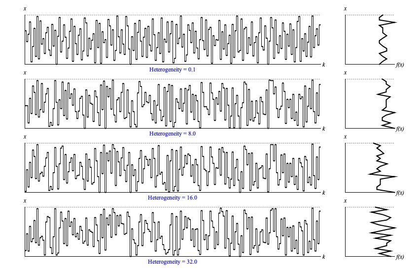
Figure 1: Sample output from Balance.next(). The left graph displays samples in time-series while the right graph presents a histogram analyzed from the same samples.

The vertical x axes for both graphs represent the driver domain from zero to unity; the horizontal k axis of the time-series graph (left) plots ordinal sequence numbers; the horizontal f(x) axis of the histogram (right) plots the relative concentration of samples at each point in the driver domain. The main takeaway from Figure 1 is that sample values are spread uniformly from zero to unity.

The topmost sequence in Figure 1 uses a heterogeneity setting of 0.1, which engages randomness only when set and clear are equally balanced. There's jaggedness in the histogram, yes, but with an average of 10 samples per histogram region the jags represent differences of mostly 1-2 samples (10-20%).

I reran these graphs several times, and it took a heterogeneity setting of 8 to make the second graph appreciably different from the first. Even here the difference is subtle. The topmost sequence alternates rapidly between low (0.0 to 0.5) and high (0.5 to 1.0) sample values. However if you look about 1/3 of the way through the second graph, you'll discover a subsequence of nine samples all lingering in the upper half of the driver domain.

Thus increasing the heterogeneity setting has the effect of stretching things out so that rather than striving for uniformity over the short term, Balance strives for uniformity over the medium term.

Bitwise Analysis

Figure 2 takes the sequence shown in Figure 1 and breaks out what happens in bit 1 (zero or one-half), bit 2 (zero or one-quarter), bit 3 (zero or one-eighth), bit 4 (zero or one-sixteenth), and the residual bits (continuous between zero and one-sixteenth).

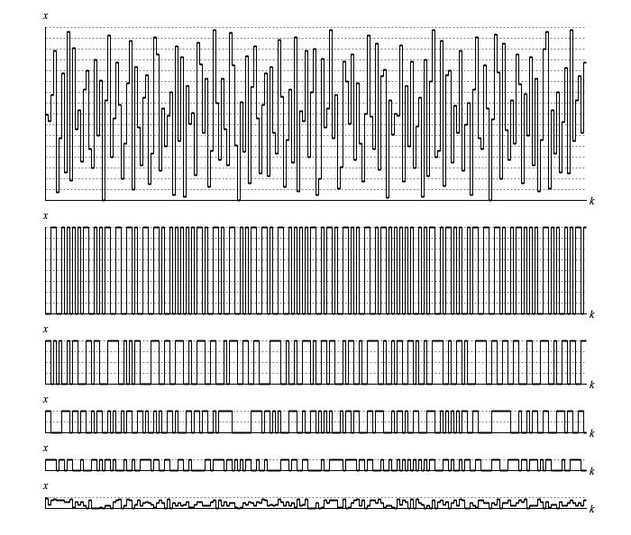
Figure 2: Bitwise analysis of a sequence generated by Balance.next().

The bit-specific graphs in Figure 2 transition back and forth between a set state (bit value 1) and a clear state (bit value 0). Table 1 statistically analyses the actual transition stats for these bit-specific graphs. Pay the closest attention to bit 1 (top row), which has just one statistic guiding its decisions. Here the number of samples between transitions is either 1 or 2, never more. That makes sense considering that for the first sample it's a coin toss, for the second sample it's the one not chosen for the first, for the third sample it's again a coin toss, for the fourth sample it's the one not chosen for the third. The other bits are more complicated. You can see for bit 2 there's never more than 4 samples between a transition; presumably for bit 3 there's never more than 8 samples between a transition.

Figure 3: Histogram of sample-to-sample differences from Balance.next() after 10,000 consecutive samples.

Transitions

Figure 3 plots the range of sample-to-sample differences along the vertical Δx axis against the relative concentrations of these values along the horizontal f(Δx) axis. Here's the reality: The Balance driver likes to jump around. The peak around zero that appears for the other probabilistic drivers — Lehmer, Borel, Moderae, Brownian, and Rosy, and Voss — is replaced in this graph by a pronounced void. The standard deviation of Δx around zero is 0.482, which well exceeds the 0.410 deviation found for the Lehmer driver — an indication of proximity aversion.

Figure 4: Divergence of 4-nibble pattern counts from Balance.next() with 10,000 samples per pattern.

Independence

Figure 4 presents a trend graph of histogram tallies for 4-nibble patterns generated using Balance.next(). My analysis program decided to exclude low-frequency patterns by limiting the graph to the 16,200 largest tallies, and since it took a long time to run I chose not to rerun with this feature disabled. The most frequent patterns were:

7	0	13	4
3	0	12	8
10	14	4	9
1	10	3	4

All of which had comparable tallies representing less than 1% presence. The distinguishing feature of these patterns is that they all contain large leaps. I don't believe there is anything special distinguishing these four patterns from any of the others that contributed to the bottom-most stair step in Figure 4.

The conclusion from Figure 4 is that the Balance driver fails the 4-nibble independence test.

/**
 * Instances of the {@link Balance} class generate a driver sequence using the balanced-bit method.
 * <p>
 * For more information including a graph of balanced-bit output, see <a href="http://www.jstor.org/stable/1513211"><i>A Catalog of Sequence Generators</i>, 1992</a>.
 * </p>
 * @author Charles Ames
 */
public class Balance extends DriverBase {
   private double heterogeneity;
   private int depth;
   private double allStats[][];
   private double scale;
   /**
    * Constructor for {@link Balance} instances with container.
    * @param container An entity which contains this driver.
    */
   public Balance(WriteableEntity container) {
      super(container);
      depth = 0;
      try {
         setDepth(6);
      } catch (Exception e) {
         throw new RuntimeException(e.getMessage(), e);
      }
      heterogeneity = Double.NaN;
   }
   /**
    * Constructor for {@link Balance} instances without container.
    */
   public Balance() {
      this(null);
   }
   /**
    * Setter for {@link #depth}.
    * @param depth The intended depth value.
    * @throws IllegalArgumentException when the argument is not positive.
    */
   public void setDepth(int depth) {
      checkDepth(depth);
      if (depth != this.depth) {
         this.depth = depth;
         int k = 1;
         allStats = new double[depth][];
         for (int level = 0; level < depth; level++) {
            double[] levelStats = new double[k];
            for (int i = 0; i < k; i++) levelStats[i] = 0;
            allStats[level] = levelStats;
            k += k;
         }
      }
      scale = Math.pow(2, depth + 1);
   }
   /**
    * Check if the indicated value is suitable for {@link #depth}.
    * @param depth The indicated value;
    */
   public void checkDepth(int depth) {
      if (0 >= depth)
         throw new IllegalArgumentException("Depth not positive");
   }
   /**
    * Getter for {@link #depth}.
    * @return The assigned {@link #depth} value.
    * @throws UninitializedException when {@link #depth} has not been initialized.
    */
   public int getDepth() {
      if (Integer.MIN_VALUE == depth) throw new UninitializedException("Depth not initialized");
      return depth;
   }
   /**
    * Setter for {@link #heterogeneity}.
    * @return The assigned {@link #heterogeneity} value.
    * @throws UninitializedException when {@link #heterogeneity} has not been initialized.
    */
   public double getHeterogeneity() {
      if (Double.isNaN(heterogeneity)) throw new UninitializedException("Heterogeneity not initialized");
      return heterogeneity;
   }
   /**
    * Getter for {@link #heterogeneity}.
    * @param heterogeneity The intended {@link #heterogeneity} value.
    * @throws IllegalArgumentException when the value is not positive.
    */
   public void setHeterogeneity(double heterogeneity) {
      checkHeterogeneity(heterogeneity);
      this.heterogeneity = heterogeneity;
   }
   /**
    * Check if the indicated value is suitable for {@link #heterogeneity}.
    * @param heterogeneity The indicated value.
    */
   public void checkHeterogeneity(double heterogeneity) {
      if (heterogeneity < MathMethods.TINY)
         throw new IllegalArgumentException("Heterogeneity must be positive");
   }
   @Override
   protected double generate() {
      int i = 0;
      int j = 0;
      int depth = getDepth();
      Random random = getRandom();
      double heterogeneity = getHeterogeneity();
      for (int level = 0; level < depth; level++) {
         double[] levelStats = allStats[level];
         double s = levelStats[j];
         double u = heterogeneity * (random.nextDouble() - .5);
         double chooser = s + u;
         int inc;
         if (chooser < 0.) {
            i++;
            levelStats[j] += 1.;
            inc = 0;
         }
         else {
            levelStats[j] -= 1.;
            inc = 1;
         }
         j = (j << 1) + inc;
         i <<= 1;
      }
      return (i + random.nextDouble()) / scale;
   }
}

Comments

1. The present text is adapted from my Leonardo Music Journal article from 1992, "A Catalog of Sequence Generators". The heading is "Balanced Bits", p. 61.
2. Statistical feedback is explained in my Perspectives of New Music article from 1990, "Statistics and Compositional Balance".