Proximate Randomness: Borel¹

Introduction

The Borel driver produces sequences which favor smaller sample-to-sample transitions over larger ones. It imposes a condition of equal probability (like a coin flip) for upward versus downward motion. A second step generates a sample uniformly in the selected region (upward or downward).

When describing the mechanism selecting consecutive section densities in his Stochastic Music Program, Iannis Xenakis expressed "a certain concern for continuity",². He also presented a formula which amounts a straight line running from a maximum for the narrowest transitions down to zero for the widest transitions. Now my page covering the Lehmer driver demonstrates that the straight-line distribution of sample-to-sample transitions in fact characterizes the standard random-number generator. However John Myhill asserted in 1979³ that the mechanism actually used in Xenakis's program was the process just described, which Myhill attributed to Émile Borel. This page shows below that this process does indeed exhibit a certain concern for continuity.

The Borel process is one of several approaches to generating sequences which exert control over distances between consecutive samples. Others include Moderate, which John Myhill suggested as an alternative to Borel, and Brownian, where control becomes parameterized.

Profile

Figure 1 illustrates Borel output with a sequence of 200 samples generated with a random seed of 1.

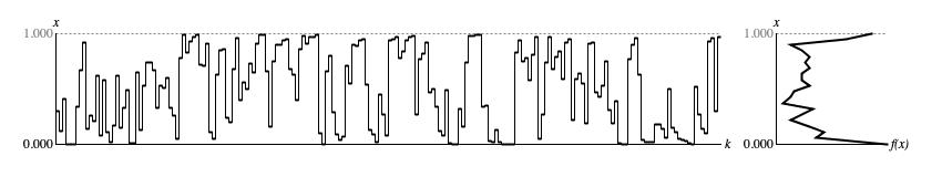
Figure 1: Sample output from Borel.next(). The left graph displays samples in time-series while the right graph presents a histogram analyzed from the same samples.

The vertical x axes for both graphs represent the driver domain from zero to unity; the horizontal k axis of the time-series graph (left) plots ordinal sequence numbers; the horizontal f(x) axis of the histogram (right) plots the relative concentration of samples at each point in the driver domain.

Bitwise Analysis

Figure 2 takes the sequence shown in Figure 1 and breaks out what happens in bit 1 (zero or one-half), bit 2 (zero or one-quarter), bit 3 (zero or one-eighth), bit 4 (zero or one-sixteenth), and the residual bits (continuous between zero and one-sixteenth).

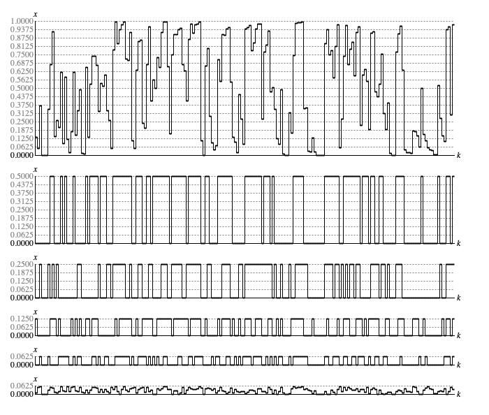
Figure 2: Bitwise analysis of a sequence generated by Borel.next().

The bit-specific graphs in Figure 2 transition back and forth between a set state (bit value 1) and a clear state (bit value 0). Table 1 statistically analyses of sample the actual stats for these bit-specific graphs. By comparison with the equivalent table for the Lehmer driver, probability has shifted away from single samples between transitions toward multiple samples between transitions.

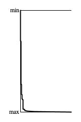
Figure 3: Histogram of sample-to-sample differences from Borel.next() after 10,000 consecutive samples.

Transitions

Figure 3 plots the range of sample-to-sample differences along the vertical Δx axis against the relative concentrations of these values along the horizontal f(Δx) axis. Difference amounts concentrate much more narrowly around zero than they did for the Lehmer driver. However, the concentrations remain decidedly positive as Δx approaches -1 from above and as Δx approaches 1 from below. Compare these concentrations to the the Moderate driver, which hugs very closely to zero at these extremes. The standard deviation of Δx around zero is 0.353, which is well short of the 0.410 deviation found for the Lehmer driver and which thus gives an indication of proximity dependence.

Figure 4: Divergence of 4-nibble pattern counts from Borel.next() with 10,000 samples per pattern.

Independence

Figure 4 presents a trend graph of histogram tallies for 4-nibble patterns generated using Borel.next(). My first attempt to produce this graph following the methods used for the Lehmer driver flatlined with negligible tallies at all points. To obtain a nontrivial result it was necessary to limit the graph the 200 largest tallies. The most frequent pattern was 0 0 0 0, representing 2% of instances. Almost as frequent was the pattern 15 15 15 15, which also had a 2% presence. Following with some 0.5% presence were the patterns 1 0 0 0 and 14 15 15 15. These details are consistent with the histogram on the right side of Figure 2, which has samples concentrating at the bottom and top of the driver range.

The glaring conclusion from Figure 4 is that the Borel driver fails the 4-nibble independence test, and does so dramatically.

/**
 * Instances of the {@link Borel} class generate a driver sequence
 * using Emile Borel's method of moderated randomness.
 * @author Charles Ames
 */
public class Borel extends DriverBase {
   /**
    * Constructor for {@link Borel} instances with container.
    * @param container An entity which contains this driver.
    */
   public Borel(WriteableEntity container) {
      super(container);
   }
   /**
    * Constructor for {@link Borel} instances without container.
    */
   public Borel() {
      this(null);
   }
   @Override
   protected double generate() {
      Random random = getRandom();
      double value = getValue();
      if (.5 < random.nextDouble()) {
         value = value * random.nextDouble();
      }
      else {
         value = value + (1. - value) * random.nextDouble();
      }
      return value;
   }
}

Comments

1. The present text is adapted from my Leonardo Music Journal article from 1992, "A Catalog of Sequence Generators". The discussion occurs on p. 62, but is missing a heading. Also the BOREL and MODERATE algorithms were reversed.
2. Iannis Xenakis, "Free Stochastic Music by Computer", chapter V of Formalized Music, page 36.
3. John Myhill, "Some Simplifications and Improvements in the Stochastic Music Program".