Controllable Proximity: Brownian¹

Introduction

The Brownian driver emulates jittery motion first observed under the microscope by biologist Robert Brown. The mathematical process which models kind of motion is "important and central" to the field of stochastic processes, which studies chains of random events. According to Wikipedia, this process was originally developed to model price fluctuations in financial markets and only later was applied (by Albert Einstein) to explain Brown's observations.

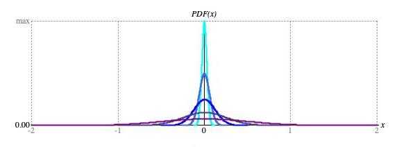
━ 1/2, ━ 1/4, ━ 1/8, ━ 1/16, ━ 1/32
Figure 5: Graphs of bell-curve (Normal) distributions centered around zero with deviation parameters
ranging from 1/2 (lowest peak, widest spread) through 1/32 (highest peak, narrowest spread).

The Brownian driver exerts parameterized control over distances between consecutive samples. More precisely, the distance Δx_k = x_k − x_k-1 is a random value distributed in a Normal distribution or bell curve such as the ones illustrated in Figure 5. The 'jitteryness' of motion depends upon the deviation, which controls how steeply probabilities roll off as Δx either increases positively from zero or decreases negatively from zero. Large deviations — for example, the purple curve in Figure 5 has deviation 1/2 — produce very active sequences while small deviations — for example, the aquamarine curve in Figure 5 has deviation 1/32 — produce more subdued motion.

Left to itself, the process just described observes no boundaries. However values from Driver.next() are required not to stray out the bounds from zero to unity. To satisfy this requirement, some containment mechanism is necessary:

• The most obvious approach is to let the process go where it will, then rescale the sequence in its entirety. The rescaling approach is not an option for Driver.next(), where contextual awareness is limited to what happened previously. An alternative method, Brownian.raw(), generates uncontained Brownian sequences. These can be captured either in a Double array or a List<Double> collection, rescaled, and then input as a source to a DriverSequence unit.
• A first Driver.next()-compliant option is use modular arithmetic to wrap x_k values outside the driver domain back into the domain. This wrapping option makes sense when the application range is cyclic; for example, a clock time, a degree of a musical scale which cycles at the octave, or a position on a color wheel. The wrapping option makes no sense at all when the application range is non-cyclic, since in this circumstance a severe discontinuity will result each time a domain boundary is crossed.
• A second Driver.next()-compliant option is reflect x_k values back from the boundaries, to the same extent that the value would have traveled if it had been allowed to cross. The reflecting option corresponds to what happens in nature, where jittering particles invariably move within some sort of container.

Other drivers concerned with distances between consecutive samples include the Borel and Moderate drivers. These two are in my mind obviated by Brownian.

Profile

Figure 1 (a) illustrates five examples of Brownian output with a sequence of 200 samples generated. All five examples were generated using a random seed of 1, an initial value of 0.5, and ContainmentMode.WRAP. The only difference is the deviation parameter, which varies as indicated.

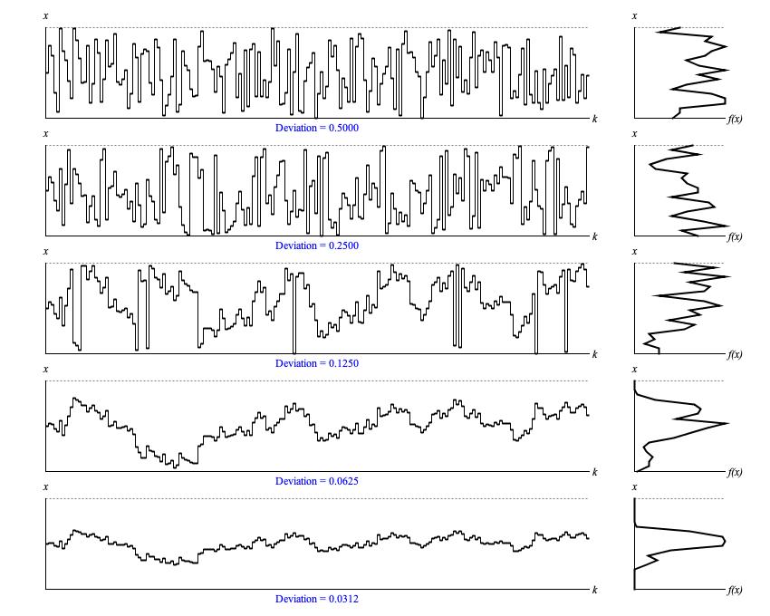
Figure 1 (a): Sample output from Brownian.next() with representative deviation settings. The left graph in each row displays samples in time-series while the right graph in the same row presents a histogram analyzed from the same samples.

The vertical x axes for the two graphs in each row represent the driver domain from zero to unity; the horizontal k axis of the time-series graph (left) plots ordinal sequence numbers; the horizontal f(x) axis of the histogram (right) plots the relative concentration of samples at each point in the driver domain.

Notice that it is not until the fourth sequence, with the deviation parameter dialed down to 1/16 of the driver range, that the sequence becomes entirely free of containment events. Even deviations this narrow cannot assure that the sequence will not ultimately stray across boundaries. The fact that this does not happen here is partly due to beginning at the dead center of the driver range. The fifth and final sequence (1/32 of the driver range) closely resembles the fourth sequence. Both share the same progression of up and down movements; the only difference in shape being one of vertical scale. This should not be surprising given that the fourth and fifth sequences both started with the same value and the same random seed.

Figure 1 (b) illustrates the difference in effect between the two containment modes. For both sequences the starting value is 0.5, the random seed is 1, and deviation is 1/8 — same as the middle sequence in Figure 1 (a). Of the two sequences pictured, the upper uses ContainmentMode.WRAP and produces exactly the same results as before. The lower sequence uses ContainmentMode.REFLECT.

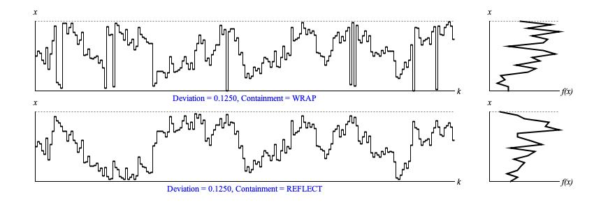
Figure 1 (b): Sample output from Brownian.next(). The left graph displays samples in time-series while the right graph presents a histogram analyzed from the same samples.

One might expect that ContainmentMode.REFLECT will flip those whole portions of the sequence which stray above unity back down under the x = 1 horizontal, but that's not what happens. Consider sequence elements 11, 12, and 13. In the fourth and fifth rows of Figure 1 (a), the sequence begins with an upward reach, then descends in two small steps. In the top row of Figure 1 (b), these three values threaten to cross the upper boundary; so all three are wrapped down into the bottom of the driver domain. However the bottom row of Figure 1 (b) applies a different containment mechanism. The value x₁₁ threatens to cross over, so it indeed is reflected. However the two small steps proceed from the reflected x₁₁ value.

If you prefer the reflect-mode behavior that flips whole portions you can substitute

Bitwise Analysis

Figure 2 takes the sequence shown for deviation 1/16 (0.0625) in Figure 1 (a) and breaks out what happens in bit 1 (zero or one-half), bit 2 (zero or one-quarter), bit 3 (zero or one-eighth), bit 4 (zero or one-sixteenth), and the residual bits (continuous between zero and one-sixteenth).

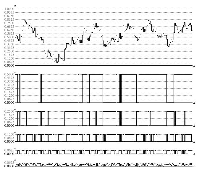
Figure 2: Bitwise analysis of a sequence generated by Brownian.next().

The bit-specific graphs in Figure 2 transition back and forth between a set state (bit value 1) and a clear state (bit value 0). Table 1 statistically analyses of sample the actual stats for these bit-specific graphs. By comparison with the equivalent table for the Lehmer driver, probability has shifted away from single samples between transitions toward multiple samples between transitions.

Transitions

Figures 3 (a) through 3 (e) plot the range of sample-to-sample differences along the vertical Δx axis against the relative concentrations of these values along the horizontal f(Δx) axis. Each graph analyzes the results of 10,000 consecutive samples generateted using ContainmentMode.REFLECT.

Figure 3 (a): Histogram of sample-to-sample differences from Brownian.next() with deviation 0.5.

Figure 3 (b): Histogram of sample-to-sample differences from Brownian.next() with deviation 0.25.

Figure 3 (c): Histogram of sample-to-sample differences from Brownian.next() with deviation 0.125.

Figure 3 (d): Histogram of sample-to-sample differences from Brownian.next() with deviation 0.0625.

Figure 3 (e): Histogram of sample-to-sample differences from Brownian.next() with deviation 0.03125.

Table 2 compares deviation parameter settings with measured deviations for Δx around zero.

Large deviation parameter settings require a lot more intervention by the containment algorithm, hence the measured deviations fall short of their parameter settings. As the parameter settings are reduced, the measured deviations come into closer and closer agreement. The correlation is less evident for ContainmentMode.WRAP.

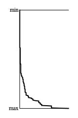
Figure 4: Divergence of 4-nibble pattern counts from Brownian.next() with deviation 0.0625 after 10,000 samples per pattern.

Independence

Figure 4 presents a trend graph of histogram tallies for 4-nibble patterns generated using Brownian.next(). My analysis program decided to exclude low-frequency patterns by limiting the graph to the 4,096 largest tallies. The most frequent patterns were:

13	13	13	13
3	3	3	3
5	5	5	5
7	7	7	7

All of which had comparable tallies representing less than 1% presence. The distinguishing feature of these patterns is that they present the same value in sequence, which means that the output stayed within 1/16 of the driver domain for four consecutive samples. I don't believe there is anything special distinguishing these four patterns from any of the others that contributed to the bottom-most stair step in Figure 4.

The conclusion from Figure 4 is that the Brownian driver fails the 4-nibble independence test.

/**
 * Generate a Brownian driver sequence with open-ended number of values.
 * @author Charles Ames
 */
public class Brownian extends DriverBase {
   /**
    * Root-mean-square distance between consecutive samples.
    */
   private double deviation;
   /**
    * Option for handling out-of-range values.
    */
   private ContainmentMode containmentMode;
   /**
    * Singleton {@link ContinuousDistribution} instance of a standard
    * bell curve centered around zero with unit deviation.
    */
   private ContinuousDistribution normalDistribution;
   private double rawValue;
   /**
    * Constructor for {@link Brownian} instances with container.
    * @param container An entity which contains this driver.
    */
   public Brownian(WriteableEntity container) {
      super(container);
      this.normalDistribution
         = ContinuousDistribution.getNormalDistribution();
      this.deviation = Double.NaN;
      this.containmentMode = null;
      this.rawValue = Double.NaN;
   }
   /**
    * Constructor for {@link Brownian} instances without container.
    */
   public Brownian() {
      this(null);
   }
   /**
    * Getter for {@link #containmentMode}.
    * @return The assigned {@link #containmentMode} value.
    */
   public ContainmentMode getMode() {
      if (null == containmentMode)
         throw new UninitializedException("Mode not initialized");
      return containmentMode;
   }
   /**
    * Setter for {@link #containmentMode}.
    * @param containmentMode The intended {@link #containmentMode} value.
    * @return True if the containment mode has changed; false otherwise.
    */
   public boolean setMode(ContainmentMode containmentMode) {
      if (this.containmentMode != containmentMode) {
         this.containmentMode = containmentMode;
         makeDirty();
         return true;
      }
      return false;
   }
   /**
    * Getter for {@link #deviation}.
    * @return The assigned {@link #deviation} value.
    */
   public double getDeviation() {
      if (Double.isNaN(deviation))
         throw new UninitializedException("Deviation not initialized");
      return deviation;
   }
   /**
    * Setter for {@link #deviation}.
    * @param deviation The intended {@link #deviation} value.
    * @return True if the deviation has changed; false otherwise.
    * @throws IllegalArgumentException when the argument is not positive.
    */
   public boolean setDeviation(double deviation) {
      if (deviation < MathMethods.TINY)
         throw new IllegalArgumentException("Deviation not positive");
      if (this.deviation != deviation) {
         this.deviation = deviation;
         makeDirty();
         return true;
      }
      return false;
   }
   /**
    * Check if the indicated value is suitable for {@link #deviation}.
    * @param deviation The indicated value.
    */
   public void checkDeviation(double deviation) {
      if (deviation < MathMethods.TINY)
         throw new IllegalArgumentException("Deviation not positive");
   }
   @Override
   protected double generate() {
      if (!Double.isNaN(rawValue)) throw new UnsupportedOperationException("Calls to next() may not intermingle with calls to raw()");
      double value = getValue();
      double change = calculateChange();
      value += change;
      return getMode().contain(value);
   }
   private double calculateChange() {
      double u = getRandom().nextDouble();
      double change = getDeviation() * normalDistribution.quantile(u);
      return change;
   }
   /**
    * Returns the next uncontained value from the driver sequence.
    * @return An unbounded real number.
    */
   public double raw() {
      if (Double.isNaN(rawValue)) rawValue = getValue();
      double change = calculateChange();
      rawValue += change;
      return rawValue;
   }
}

Comments

1. The present text is adapted from my Leonardo Music Journal article from 1992, "A Catalog of Sequence Generators". The heading is "Brownian Motion", p. 62.