Proximate Randomness: Voss¹

Introduction

The Voss driver produces sequences which reputedly emulate 1/f noise. Each sample value is the sum of N sample-and-hold streams, where N is a user-selected parameter implemented as Voss.depth. The decision of whether a given stream should sample (obtain a new value from java.util.Random.nextDouble()) or hold (retain the previous stream value) happens for every sample in stream 0, for every other sample in stream 1, for every third sample in stream 2, and for every k+1st sample for stream k.

The Voss process is one of several approaches to generating sequences which exert control over distances between consecutive samples. Others include Brownian and Rosy.

Profile

Figure 1 illustrates Voss output with five sequences of 200 samples generated with varying sample-and-hold stream counts.

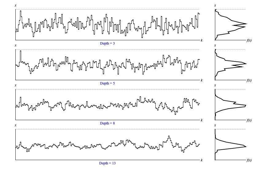
Figure 1: Sample output from Voss.next(). For each row of graphs, the leftward graph displays samples in time-series while the rightward graph presents a histogram analyzed from the same samples.

The vertical x axes for both graphs represent the driver domain from zero to unity; the horizontal k axis of the time-series graph (left) plots ordinal sequence numbers; the horizontal f(x) axis of the histogram (right) plots the relative concentration of samples at each point in the driver domain.

Probability theory has an insight called the Central Limit Theorem which asserts that as N increases, adding together N random variables with mean μ and deviation σ will produce a bell curve centered around Nμ with deviation √Nσ. Since the held samples in one stream range uniformly from zero to unity, each stream has mean μ = 0.5 and deviation σ = √12 = 0.29. Since the sequences in Figure 1 present the average of all sample-and-hold streams, the bell curve will be centered around Nμ/N = μ = 0.5 and its the deviation around this center will be √Nσ/N = σ/√N = 0.29/√N.

The limiting case of depth = 1 is standard randomness of Lehmer. As depth increases, values cluster ever-more closely around 0.5, converging ultimately to a flat line.

Bitwise Analysis

Figure 2 takes the sequence shown in the second row Figure 1 and breaks out what happens in bit 1 (zero or one-half), bit 2 (zero or one-quarter), bit 3 (zero or one-eighth), bit 4 (zero or one-sixteenth), and the residual bits (continuous between zero and one-sixteenth).

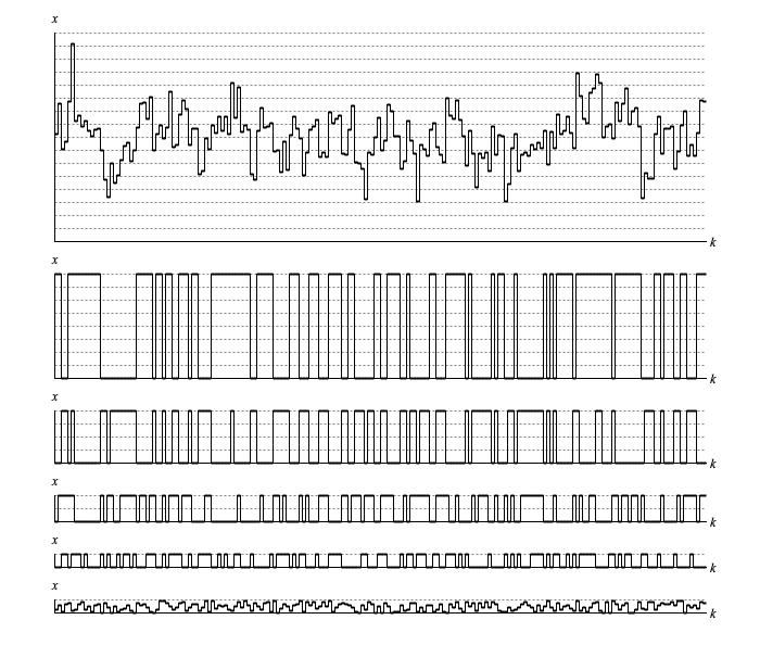
Figure 2: Bitwise analysis of a sequence generated by Voss.next()for depth = 5.

The bit-specific graphs in Figure 2 transition back and forth between a set state (bit value 1) and a clear state (bit value 0). Table 1 statistically analyses of sample the actual stats for these bit-specific graphs. By comparison with the equivalent table for the Lehmer driver, probability has shifted away from single samples between transitions toward multiple samples between transitions.

Transitions

Figures 3 (a) through 3 (d) plot the range of sample-to-sample differences along the vertical Δx axis against the relative concentrations of these values along the horizontal f(Δx) axis.

Figure 3 (a): Histogram of sample-to-sample differences from Voss.next() with depth 3 after 10,000 consecutive samples.

Figure 3 (b): Histogram of sample-to-sample differences from Voss.next() with depth 5 after 10,000 consecutive samples.

Figure 3 (c): Histogram of sample-to-sample differences from Voss.next() with depth 8 after 10,000 consecutive samples.

Figure 3 (d): Histogram of sample-to-sample differences from Voss.next() with depth 13 after 10,000 consecutive samples.

Table 2 compares depth parameter settings with measured deviations for Δx around zero.

Independence

Figure 4 presents a trend graph of histogram tallies for 4-nibble patterns generated using Voss.next() with depth = 5. The most frequent patterns were:

All of which had comparable tallies representing less than 1% presence. The distinguishing feature of these patterns is that they concentrate in the middle 2/16ths of the driver range.

The conclusion from Figure 4 is that the Brownian driver fails the 4-nibble independence test.

/**
 * Instances of the {@link Voss} class generate a 1/f driver
 * sequence using the algorithm of Richard Voss.
 * @author Charles Ames
 */
public class Voss extends DriverBase {
   /**
    * Facts concerning an individual sample-and-hold stream.
    * @author Charles Ames
    */
   protected class Partial {
      double increment;
      double phase;
      double value;
      protected Partial() {
         /**
          * Whenever this value exceeds unity, resample
          * then wrap back into range from zero to unity.
          */
         phase = Double.NaN;
         /**
          * Controls the resampling rate.  Add this to
          * the phase each cycle, before determining whether
          * to resample.
          */
         increment = Double.NaN;
         /**
          * Holds random sample value.
          */
         value = Double.NaN;
      }
   }
   /**
    * Number of sample-and-hold streams.
    */
   private int depth;
   /**
    * Resampling-rate exponent.
    */
   private boolean valid;
   private List<Partial> partials;
   /**
    * Constructor for {@link Voss} instances with container.
    * @param container An entity which contains this driver.
    */
   public Voss(WriteableEntity container) {
      super(container);
      this.depth = Integer.MIN_VALUE;
      partials = new ArrayList<Partial>();
      valid = false;
   }
   /**
    * Constructor for {@link Voss} instances without container.
    */
   public Voss() {
      this(null);
   }
   /**
    * Getter for {@link #depth}.
    * @return The assigned {@link #depth} value.
    */
   public int getDepth() {
      if (Integer.MIN_VALUE == depth)
         throw new UninitializedException("Depth not initialized");
      return depth;
   }
   /**
    * Setter for {@link #depth}.
    * @param depth The intended {@link #depth} value.
    */
   public void setDepth(int depth) {
      checkDepth(depth);
      this.depth = depth;
      Random random = getRandom();
      partials.clear();
      double sum = 0;
      for (int index = 0; index < depth; index++) {
         Partial partial = new Partial();
         partials.add(partial);
         partial.phase = MathMethods.TINY;
         partial.increment = 1. / (index+1);
         partial.value = random.nextDouble();
         sum += partial.value;
      }
      setValue(sum/depth);
      valid = false;
   }
   /**
    * Check if the indicated value is suitable for {@link #depth}.
    * @param depth The indicated value.
    */
   public void checkDepth(int depth) {
      if (0 >= depth)
         throw new IllegalArgumentException("Invalid depth: " + depth);
   }
   protected double generate() {
      if (!valid) {
         valid = true;
      }
      Random random = getRandom();
      double sum = 0;
      for (int index = 0; index < depth; index++) {
         Partial partial = partials.get(index);
         partial.phase += partial.increment;
         if (partial.phase > 1.) {
            partial.value = random.nextDouble();
            partial.phase = partial.phase % 1.;
         }
         sum += partial.value;
      }
      return sum / depth;
   }
}

Comments

1. The present text is based on "Fractional Noise", a topic from Chapter 11, "Composition with Computers" in the 1997 book Computer Music, 2nd Edition, by Charles Dodge and Thomas Jerse, pp. 368-370.