Tone Clusters
Introduction
The Wikipedia article on Tone Clusters defines such a thing as “a musical chord comprising at least three adjacent tones in a scale”. The present page adopts a didactic approach by first evaluating clusters which fill a single octave with simple sine waves. The page goes on to consider methods by which sine-tone clusters may be extended and refined. It was hoped originally that an investigation progressing incrementally from single-octave sine clusters through multi-octave extensions and beyond would lay out a diversity of material which could then be exploited compositionally.
I began this study knowing a lot less about tone clusters than I thought I did. I was familiar with their use in pieces by composers such as Henry Cowell. I was, and remain, doctrinally sympathetic to the Emancipation of the Dissonance. I have a longstanding interest in microtonal music and had the thought that the quarter-tone clusters of Krzysztof Penderecki might provide a doorway into this topic. However while working with my Sound application to generate sound examples I encountered a rather brutal reality check.
This page adopts the principle of emphasizing all tones uniformly. This principle requires that given a certain cluster density, every tone identified by that density be represented in the cluster. So for example, a closed (one-octave) cluster with semitone density will contain twelve tones while a closed cluster with quarter-tone density will contain twenty four tones. Within the first exercise, the equal-emphasis principle also requires that every tone have equal amplitude. As the page proceeds, the requirement of equal amplitude will be generalized in various ways, and ultimately relaxed.
There is a basic commonality between the equal-emphasis principle stated here and Arnold Schoenberg's twelve-tone technique. That commonality is a selection process which conforms pitch choices to a statistical distribution, and more specifically, to a uniform distribution. However, the present page does not advocate twelve-tone ideology. Rather the equal-emphasis principle is adopted here in order to develop a central paradigm — indeed an extremity — providing other approaches with context.
Coming into this page, you should understand about tones and how they are generated. Tone generation is explained in the Waveform Reference. You should also be able to interpret a frequency-spectrum graph. These are bar graphs plotting frequency on the horizontal axis against amplitude on the vertical axis. Features of such graphs are discussed in the opening of my page on Synthesizing Noise Sounds. Most of the frequency-spectrum graphs on the present page plot amplitudes linearly, as sample magnitudes, but a few plot amplitudes logarithmically, as decibels. Most graphs plot frequencies logarithmically, in cents. A few graphs employ directly linear frequency plots.
Sine Clusters
This first exercise builds clusters in closed voicing, with tones specifically limited to the octave above middle C (261.6 Hz.). All of the tones will be generated using sine waves. A sine wave is a fundamental with no additional harmonics. Sine waves are the simplest and purest of all tones.
orch /Users/charlesames/Scratch/ToneClusterOrch.xml
set norm 1
set bits 16
set rate 44100
// Ins 1:  Tone
note 1 1 1 0 0.25 2.00 0.3485491038 261.6 1
note 2 1 1 0 0.25 2.00 0.3485491038 293.6360718377 1
note 3 1 1 0 0.25 2.00 0.3485491038 329.5953466525 1
note 4 1 1 0 0.25 2.00 0.3485491038 369.9582679168 1
note 5 1 1 0 0.25 2.00 0.3485491038 415.2641151949 1
note 6 1 1 0 0.25 2.00 0.3485491038 466.118209331 1
// Ins 5:  EnvSust
note 7 1 5 0 0.25 2.00 1000 0.03 0.1
// Ins 21:  Rebalance-Output
note 8 1 21 0 0.25 1.75
end 2.50ToneClusterOrch.xml.
Orchestra
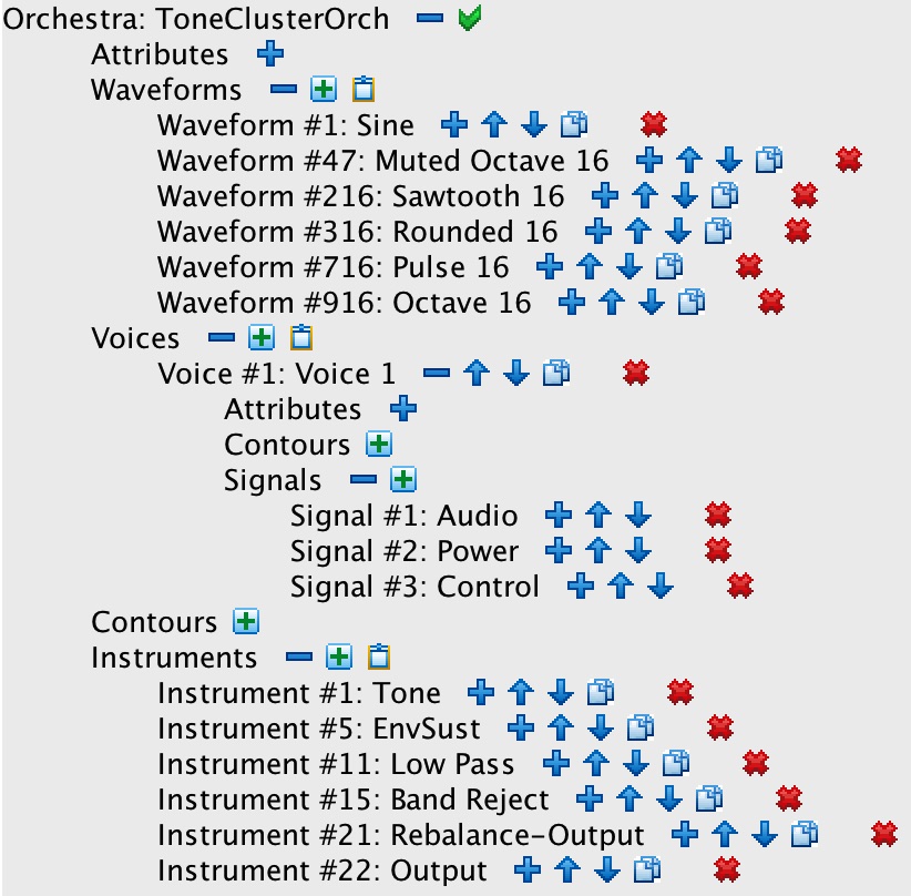
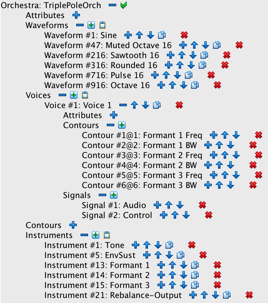
The Sound orchestra used to generate sound examples for the present exercise is outlined in Figure 1-1.
This orchestra pursues an additive model of sound synthesis
by building up complex sounds (clusters) from simple components (tones).
Notice that the orchestra defines three signals scoped to Voice #1;
these allow instruments to pass both audio and control data between notes, so long as the notes belong to the same voice.
The voice-scoped signals employed for this exercise are G1 for audio data and G3 for control
data (envelopes); voice-scoped signal #2 is not used.
Only three of the instruments listed are actually employed to generate sine clusters:
-
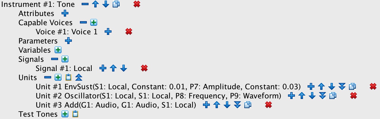
Instrument #1: Tone detailed in Figure 1-2 chains together three units:
- Unit #1 is an EnvSust (sustained envelope) looking to note parameter #7 for its peak amplitude. This unit is extra baggage in Listing 1, where tone durations coincide with overall cluster durations. However, individual envelopes become necessary when clusters are arpeggiated below.
- Unit #2 is an Oscillator generating an individual tone. The oscillator takes its amplitude from Unit #1. It looks to note parameter #8 for its frequency and to note parameter #9 for its waveform ID. The waveform ID must be one of those listed under Waveforms in Figure 1-1.
- Unit #3 is an Add operator. When applied to signals, the addition operation has the effect of mixing the signals together, thus Unit #3 mixes the tone from Unit #2 into the voice-scoped audio signal G1.
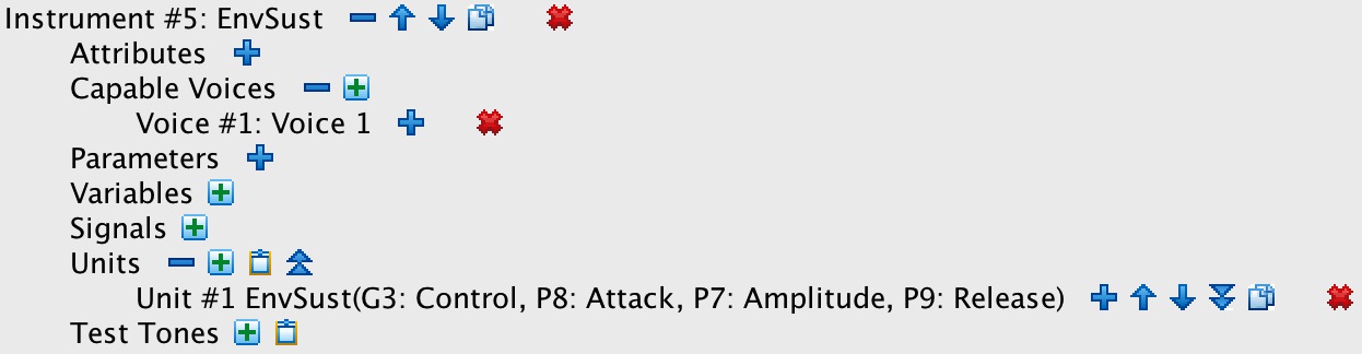
notereferencing Instrument #1: Tone; thus notes numbers 1-6 in Listing 1 together produce a whole-tone cluster. Notice that parameter #9 in each of these notes references Waveform #1: Sine in Figure 1-1.1 - Instrument #5: EnvSust detailed in Figure 1-3 employs just one unit. This is an EnvSust (sustained envelope), which generates the amplitude profile for the entire cluster. This unit outputs its the result to the voice-scoped control signal G3, which transmits the envelope to other instruments. Note #7 in Listing 1 activates Instrument #5: EnvSust to generate an envelope.
-
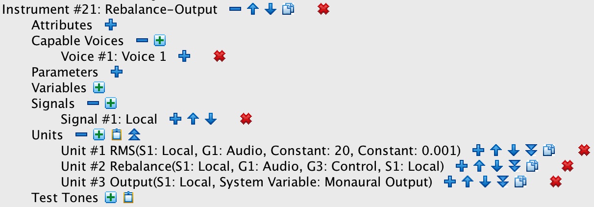
Instrument #21: Rebalance-Output detailed in Figure 1-4 employs three units:
- Unit #1 is an RMS power extractor. It extracts the audio power envelope from G1.
- Unit #2 is a Rebalance. This unit type compounds two arithmetic operations: multiplication with division. In the present case, Unit #2 multiplies the audio signal G1 by the control signal G3 and divides the result by the power envelope from Unit #1. Dividing the audio signal by its power envelope has the effect of normalizing the audio signal, that is, of suppressing or boosting the audio amplitude as required to obtain an RMS amplitude of 1. Multiplying this normalized audio signal by the envelope control has the effect of amplifying the former by the latter, imposing the shape generated by Instrument #5: EnvSust upon the audio content generated by Instrument #1: Tone.
- Unit #3 is a single-channel Output. It mixes the results from Unit #2 into the output buffer for channel #0 (the only channel available for monaural output). From which buffer the data will be written out to file.
Note-List Generation
Preparing note lists quickly becomes tiresome. Allowing notes to pass information between one another through
voice-scoped signals facilitates generating clusters comprised of any
number of tones, but this enhanced facility also increases — by an order of magnitude — the amount of information
needed to describe a sound.
Implicit in voice-scoped sound generation is the concept of an instrument stack, earlier developed on the page
Synthesizing Noise Sounds. To produce a single sound,
an instrument stack combines one or more sources, processes the combination through one or
more modifiers, and ultimately directs the result to one or more output channels. Each source, each modifier, and
output will be invoked using a note statement.
By now I have come to rely entirely on programs to handle these details. While the Sound orchestra
doesn't explicitly implement an instrument-stack entity, my note-list generating programs centralize functionality
in an InstrumentStack class. Each InstrumentStack instance manages a
collection of StackElement instances. Each StackElement instance in
turn references an instrument from the orchestra. Various StackElement subclasses implement
sets of properties, as necessary to construct notes for that particular instrument.
My InstrumentStack instance for the present exercise references the orchestra pictured in Figure 1-1
through Figure 1-4, it also has awareness that the notes it generates will belong to Voice #1.
The StackElement subclasses managed under this stack are a Cluster
element which references Instrument #1: Tone, an Envelope
element which references Instrument #5: EnvSust, and an Output
element which references Instrument #21: Rebalance-Output.
The StackElement class mandates a createNote method with three arguments: a notelist
reference, a start time and a duration. Remember that every note statement
must have a note ID (P1), a voice ID (P2), an instrument ID (P3), a slur-from ID (P4; not used for these exercises), a start time
(P5), a duration (P6), plus zero or more instrument-specific parameters. Now, the notelist itself can hand back
the next available note ID. The voice ID is known by the InstrumentStack, the instrument ID is known
by the StackElement, the slur-from ID defaults to zero; finally, the start time and duration are both
method parameters. This leaves it to the StackElement subclasses to fill in the instrument-specific
parameters.
The Cluster subclass of StackElement understands that that note statements for
Instrument #1: Tone must additionally include an amplitude (P7), a frequency (P8), and a waveform ID (P9).
In addition, Cluster is aware that separate notes are required for each tone in the cluster.
Thus Cluster
Thus Cluster itself manages a collection of Tone instances, each Tone
being described by an amplitude and a frequency.
The note-list generating program for present exercise extends stack-element subclassing with a ClosedCluster subclass
of the Cluster class.
ClosedCluster inherits have two properties from Cluster which ClosedCluster
uses to initialize its collection of tones. These properties are a lowest Pitch and a ClusterDensity
reference. There are static ClusterDensity instances for 3, 4, 6, 12, 18, 24, 36, 48, and 60 steps per
octave. Each ClusterDensity instance manages as many ClusterChroma instances as there are steps.
Properties of ClusterChroma include a step number ranging from 0 to the step count and
a frequency ratio ranging from 1 (inclusive) to 2 (exclusive).
Each of the sound examples presented in Figure 2-1 through Figure 2-9
was generated using ClosedCluster with the low pitch set to C4 (middle C), with the waveform set to
Waveform #1: Sine, and with the ClusterDensity reference set as indicated.
Sound Examples
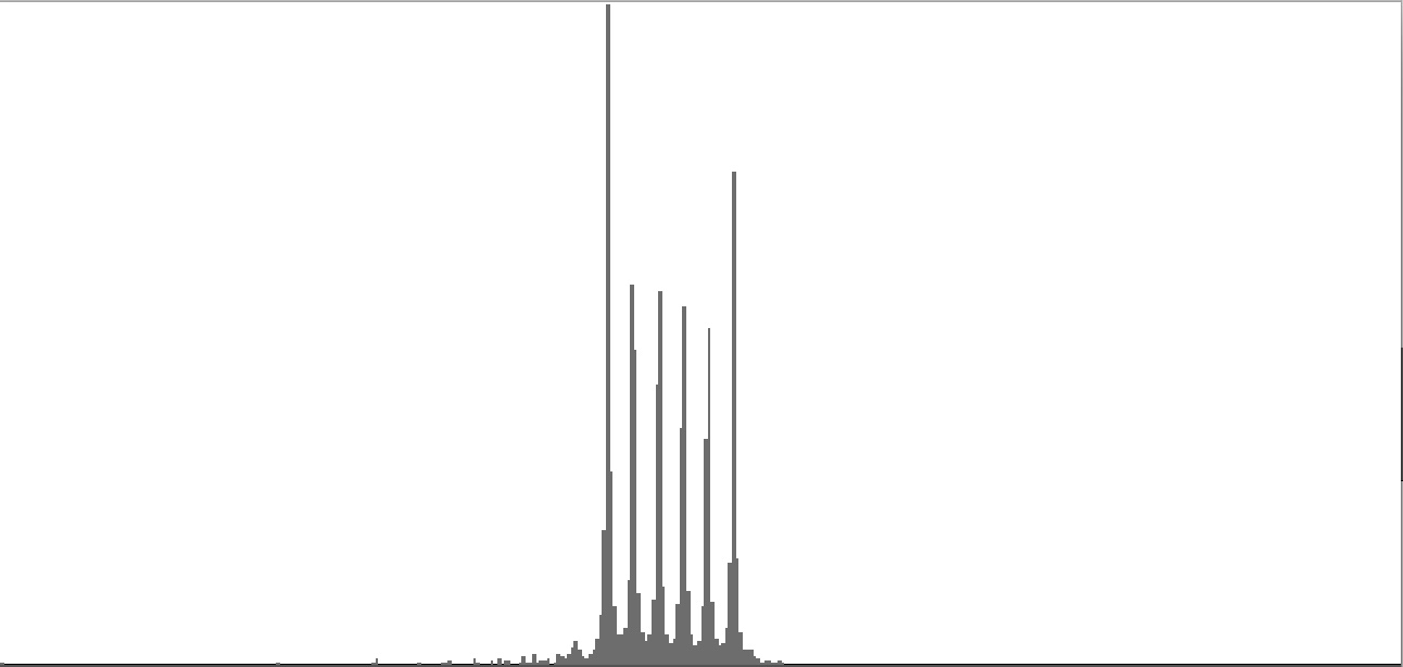
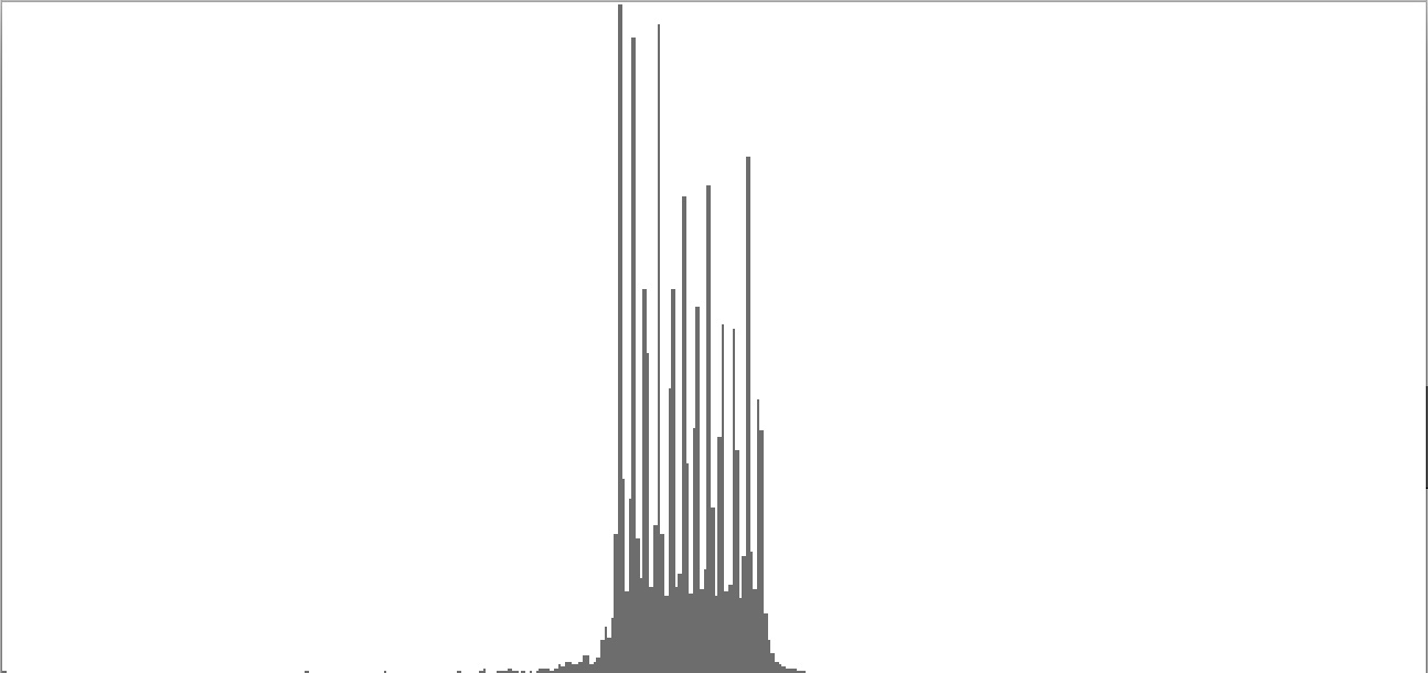
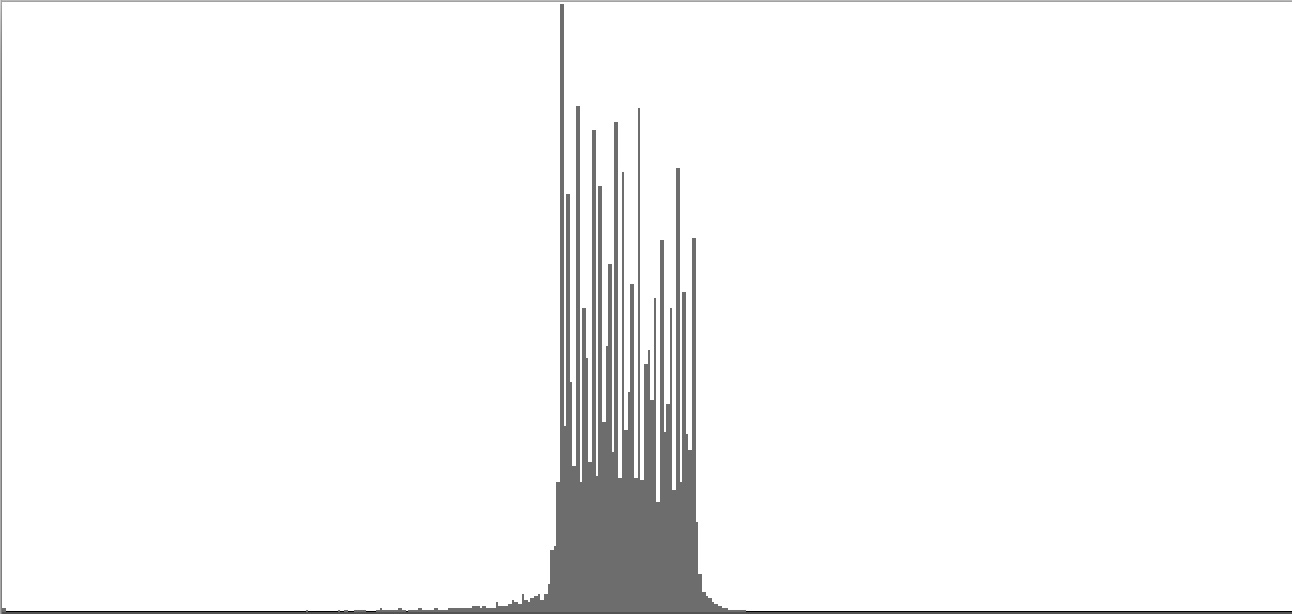
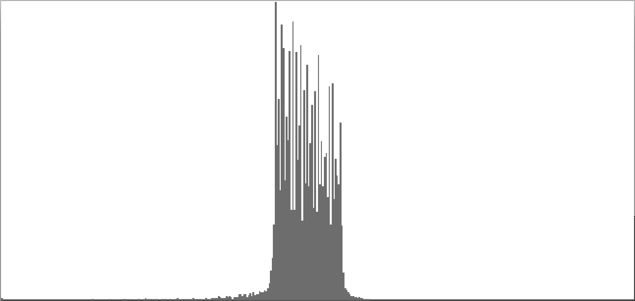
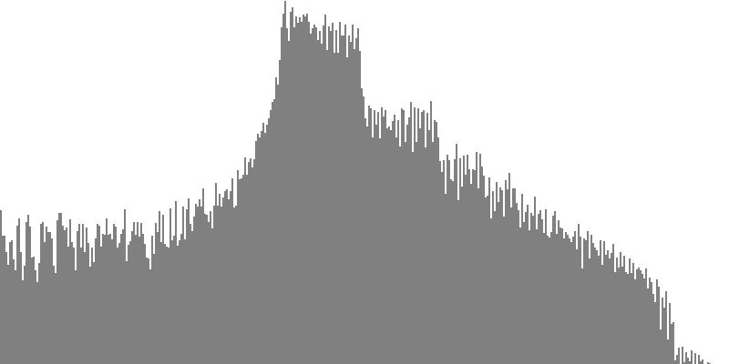
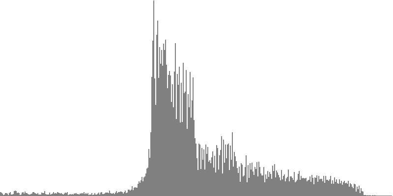
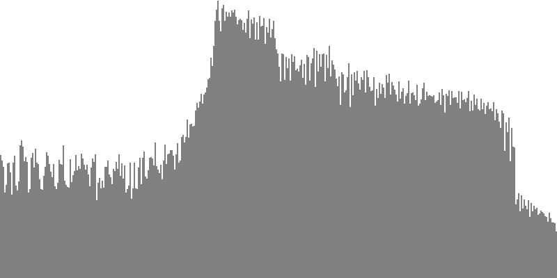
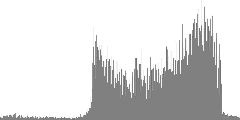
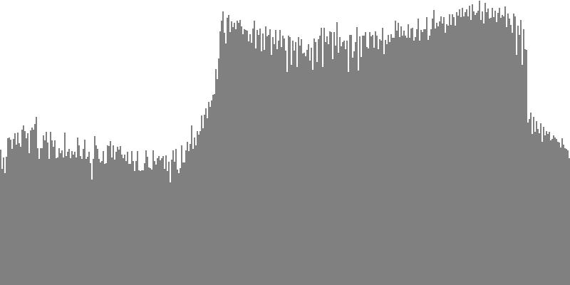
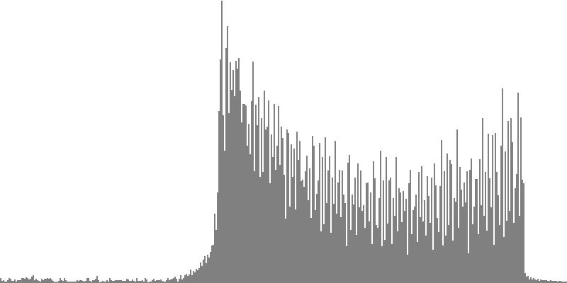
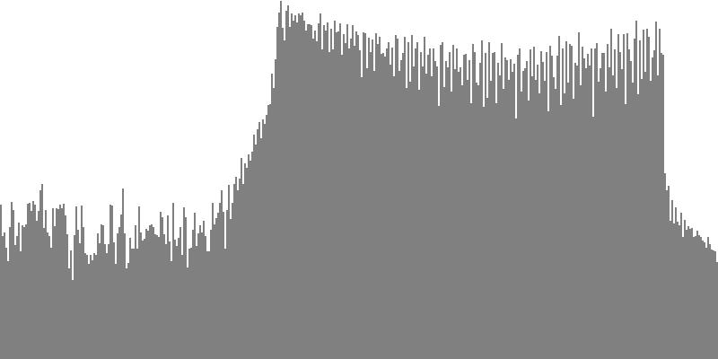
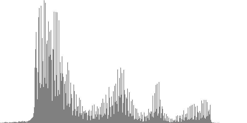
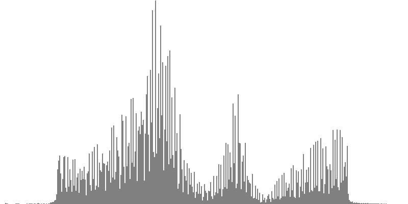
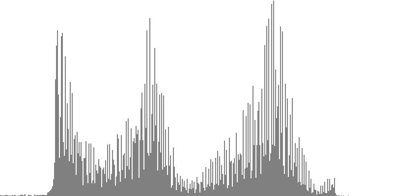
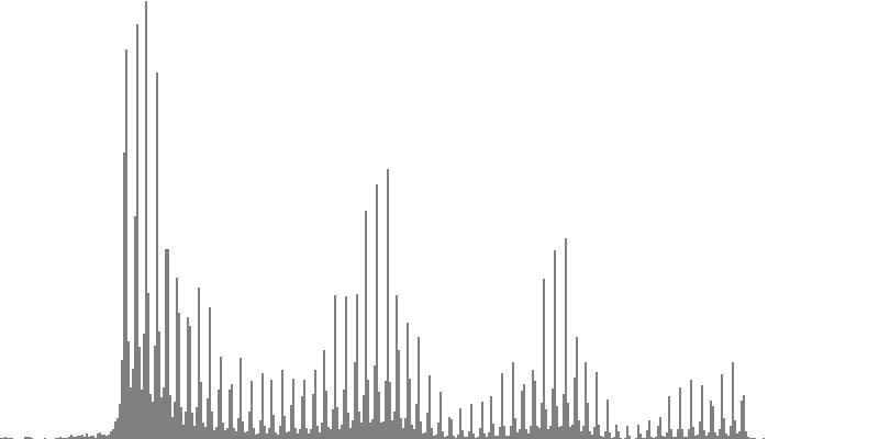
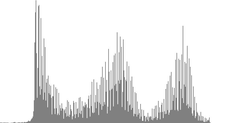
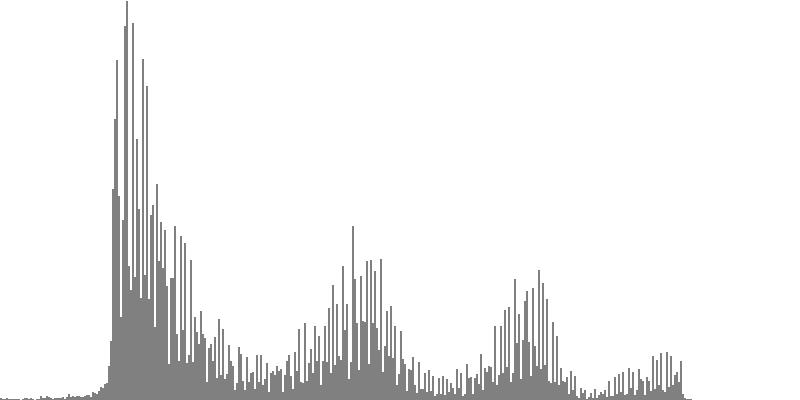
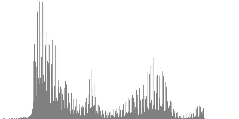
This exercise explores the point of crossover from discrete into continuous frequency spectra. Such crossover is shown graphically in the series of frequency-spectrum graphs presented as Figure 2-1 through Figure 2-9. These nine frequency-spectrum graphs were each obtained by analyzing one second of sound with 400 frequency bands whose center frequencies proceed logarithmically from 16 Hz. to 10,000 Hz.
In the discrete spectrum presented as Figure 2-1, the components of a sound resolve into discernible tones which appear as narrow spikes separated by wide gaps. In this first instance the tones form an augmented triad dividing the octave into three equal parts. By contrast, the spectrum presented as Figure 2-9 depicts a continuous noise band. You still see spikes, but there's no longer any white space between them. You certainly cannot discern tones from the sound example.

|

|
|
||
| Figure 2-1: Frequency-spectrum graph of sine-wave chord dividing the octave into 3 equal parts (augmented triad). To hear a realization, click here. | Figure 2-2: Frequency-spectrum graph of sine-wave chord dividing the octave into 4 equal parts (diminished seventh chord). To hear a realization, click here. | Figure 2-3: Frequency-spectrum graph of sine-wave cluster dividing the octave into 6 equal parts (whole-tone scale). To hear a realization, click here. | ||
|
|
|
||
| Figure 2-4: Frequency-spectrum graph of sine-wave cluster dividing the octave into 12 equal parts (chromatic scale). To hear a realization, click here. | Figure 2-5: Frequency-spectrum graph of sine-wave cluster dividing the octave into 18 equal parts (third-tone scale). To hear a realization, click here. | Figure 2-6: Frequency-spectrum graph of sine-wave cluster dividing the octave into 24 equal parts (quarter-tone scale). To hear a realization, click here. | ||
|
|
|
||
| Figure 2-7: Frequency-spectrum graph of sine-wave cluster dividing the octave into 36 equal parts (sixth-tone scale). To hear a realization, click here. | Figure 2-8: Frequency-spectrum graph of sine-wave cluster dividing the octave into 48 equal parts (eighth-tone scale). To hear a realization, click here. | Figure 2-9: Frequency-spectrum graph of sine-wave cluster dividing the octave into 60 equal parts. To hear a realization, click here. |
Let us now evaluate the first four of these sounds individually:
- Dividing the octave into three equal parts produces the augmented triad whose frequency-spectrum graph appears as Figure 2-1. Augmented triads are consonant, at least in comparison with the other sounds generated in this exercise.
- Dividing the octave into four equal parts produces the diminished seventh chord whose frequency-spectrum graph appears as Figure 2-2. Diminished seventh chords are mildly dissonant.
- Dividing the octave into six equal parts produces the whole-tone cluster whose frequency-spectrum graph appears as Figure 2-3. Whole-tone clusters are strongly dissonant.
- Dividing the octave into twelve equal parts produces the semitone cluster whose frequency-spectrum graph appears as Figure 2-4. Semitone clusters are the most dissonant sounds obtainable from standard equal temperament.
The four sounds just described predict a trend: clusters which divide the octave with ever-finer densities should produce ever-more-dissonant sounds. We test this prediction with densities of eighteen (Figure 2-5), twenty-four (Figure 2-6), thirty-six (Figure 2-7), forty-eight (Figure 2-8), and sixty (Figure 2-9) sine tones per octave. Play each sound in Figure 2-1 through Figure 2-9 in sequence and judge for yourself whether the prediction holds true.
If you're like me, you didn't hear much if any difference between densities of 18, 24, 36, 48, and 60 sine tones per octave. The explanation is probably that at around 18 tones per octave, the crossover from discrete into continuous is effected. Your ear is no longer discriminating between individual tones; rather, what you perceive is band-limited noise.
This is the reality check I was referring to in the Introduction. I have encountered the third-tone threshold in other forays into microtonal tuning; this also is the threshold where consecutive tones loose chromatic distinction and begin to be heard as mistunings of one another.
Waveform Clusters
This second exercise lowers the bottom-most pitch in the cluster to G3 (196.0 Hz.) and replaces the simple sine tones with several of the compound forms described in the Waveform Reference. For each waveform family, the four-octave variant has been employed. This would be the variant with harmonic numbers ranging up to 16. Since the upper bound for each cluster is G4 (392.0 Hz.), the highest pitch produced will be just short of G8 (6272 Hz.).
Video 1: Sonogram of sine-cluster sequence; sounds divide octave above G3 successively into 3, 4, 6, 12, 18, 24, 36, 48, and 60 equal parts.
The sound examples to follow realize sequences of clusters with 3, 4, 6, 12, 18, 24, 36, 48, and 60 equal steps to the octave. One purpose is to explore the diversity of sounds obtained by employing different waveforms. Another purpose is to determine if changing waveforms affect the point of spectral crossover from discrete to continuous. A sequence realized using pure sine waveforms appears as Video 1. This figure makes use of a capability which is new to the Sound application's wave-viewer, the sonogram. Sonograms display how frequency spectra unfold over time. Frequencies are plotted in the vertical dimension against time along the horizontal dimension. Each frequency band is represented by a single pixel, and the intensity of sound within that frequency band is indicated by a gray-scale color ranging from white (no intensity) to black (maximum intensity).
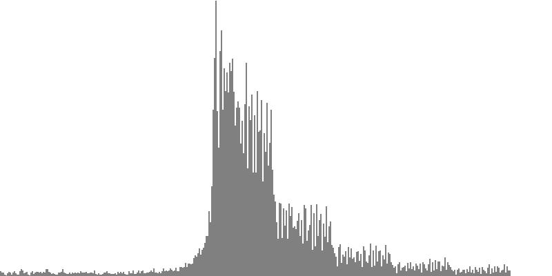
The frequency-spectrum graphs for this second exercise are presented in pairs: the first spectrum graph plots amplitudes linearly as sample magnitudes while the second spectrum graph plots amplitudes logarithmically in decibels. These paired graphs were were obtained by analyzing the same sample of sound. The analysis in each case employed 400 frequency bands with center frequencies proceeding logarithmically from 16 Hz. to 10,000 Hz.
The rounded sawtooth wave of Figure 4-1a and Figure 4-1b combines all harmonics, with amplitudes falling off with the squared inverse of the harmonic number. To hear a realized sequence with 3, 4, 6, 12, 18, 24, 36, 48, and 60 equal steps to the octave, click here.
The sawtooth wave of Figure 3-2a and Figure 3-2b combines all harmonics, with amplitudes falling off with the direct (unsquared) inverse of the harmonic number. To hear a realized sequence with 3, 4, 6, 12, 18, 24, 36, 48, and 60 equal steps to the octave, click here.
The pulse wave of Figure 3-3a and Figure 3-3b combines all harmonics with equal amplitudes. To hear a realized sequence with 3, 4, 6, 12, 18, 24, 36, 48, and 60 equal steps to the octave, click here.
The octave-doubled sine wave of Figure 3-4a and Figure 3-4b contains only harmonics whose frequency ratio with the fundamental is a power of two. All harmonics have equal amplitude. To hear a realized sequence with 3, 4, 6, 12, 18, 24, 36, 48, and 60 equal steps to the octave, click here.
The rounded, sawtooth, and pulse tone-cluster variants have no particular claim to fame. However octave-doubled sine clusters have this feature: not only do the fundamentals have equal amplitudes between G3 and G4, but the same amplitudes apply to the 2nd harmonics between G4 and G5, to the 4th harmonics between G5 and G6, and so forth to the 8th and 16th harmonics. Some of you may recognize that having equal spectral energy in all octaves is one defining feature of White Noise. Now strictly speaking, clusters don't transition into noise until they've crossed the threshold from the discrete into the continuous. Meaning 18 or more tones per octave. Also, the octave-doubled cluster presented in Figure 3-4a and Figure 3-4b is band limited White Noise, since audio ranges below G3 and above G8 are excluded.
Having a flat spectrum makes the octave-doubled sine clusters particularly suitable for driving subtractive synthesis. The rub is that white noise is extremely harsh, and extra steps may be considered necessary just to mitigate such harshness. One approach might be to carry on with the notion of noise colors. If equal-amplitude octave doubling can be used to generate white noise, then setting amplitudes to the inverse of the harmonic number should produce a reasonable approximation of Pink Noise. Likewise, setting amplitudes to the squared inverse of the harmonic number should produce a reasonable approximation of Brown Noise.
I write “approximation” in the previous paragraph because the spectrum produced steps down for each octave while the drop off should technically be gradual, as shown here. But stepping down by octave is not necessarily bad. When the first exercise generated sine-tone clusters with equal amplitudes, for example in Listing 1, the equal-emphasis principle asserted that no specific tone in the cluster was any more significant than any other. For the present muted-octave doubling, the same assertion applies.
Figure 3-5a and Figure 4-5b use the term “muted octave doubling” to describe an octave-doubled waveform with amplitudes set to the inverse of the harmonic number. To hear a realized sequence with 3, 4, 6, 12, 18, 24, 36, 48, and 60 equal steps to the octave, click here.
Arpeggiated Clusters
The previous exercise brought tone clusters across the threshold from discrete dissonance to continuous noise and ultimately attained the extreme harshness of white noise. There is no further to go along this path, so going forward this page explores ways of mitigating the harshness of tone clusters. The next two exercises continue applying the additive model of building sounds up from piles of note statements, one note for each tone. However, we now retreat from the practice of playing all the notes, all the time.
This third exercise explores a way of spinning a cluster's content out by dividing the overall duration into moments and by presenting just a subset of tones in each moment.
The present group of sound examples divides overall playing durations of 2 seconds into 16 moments of 1/8 second duration each. The number of tones playing during any one moment will be fixed at half the number of tones in the cluster; e.g. six tones for semitone clusters, nine tones for third-tone clusters, and so forth. Each tone is realized using an octave-doubled sine waveform. The equal-emphasis principle still applies; however, it does not apply to individual moments. Rather, the principle broadens out horizontally to frames of three or four moments in succession.
Note-List Generation
To decide which tones would play when, my note-list generating program employed the technique of statistical feedback.
Statistical feedback is the topic of an animated demonstration given elsewhere on this site.
The technique is a mostly determinate way of selecting resources driven by the fair-share principle.2
The classes employed by this program include Tone, Moment, Strand, and EventType.
-
The
Toneclass has been previously described as a member component whichClosedClusterinherits fromCluster. The properties ofToneinclude amplitude and frequency. The number ofToneinstances is determined by theClusterDensitystep count, which we will presently designate using the letter N. Thus for a semitone cluster N=12. OtherToneproperties are a preference value φn and a usage statistic Un; these properties will be explained below.Toneinstances are organized into an array of references, here called a schedule, which can be reordered to reflect changing preferences. -
The
Momentclass is particular to this program. Its properties include starting time and duration. We will use T to indicate the number of moments, which was previously fixed at 16. Another property ofMomentinstance t is Kt, which is the number of newly entering tones. -
The
Strandclass is also particular to this program. Instances of this class act as channels within which aToneis permitted to sound. We will use M to indicate the number ofStrandinstances, which for this third exercise sets to two thirds of theClusterDensitystep count. Thus for a semitone cluster M=12×2/3=8. AnotherStrandproperty is a dynamic count of tone-initiations.Strandinstances are also organized into a schedule, which can be reordered to reflect changing preferences. -
The
EventTypeclass is actually an enumerated type. AnEventTypecan be either aTONE_INITIATIONor aTIE.
The present note-list generating program is structured as a pair of nested loops.
An outer loop iterates through the sequence of Moment instances, while the inner loop iterates through
the schedule of Strand instances. You can imagine therefore that the program is cycling its way
through a two-dimensional grid, where each cell describes what a particular Strand is doing during
a particular Moment. The activity within a cell is described by an EventType and a
Tone reference.
Each iteration of the outer loop does three things for Moment instance t:
- The program first selects Kt, which is the number of newly entering tones. For the semitone cluster the Kt values are 6, 3, 4, 3, 2, 4, 3, 4, 3, 4, 2, 6, 2, 4, 3, 3.
-
The schedule of
Strandinstances is sorted into preference order based upon how many tone initiations have been allocated so far to each particularStrand.Strandinstances with fewer initiations occupy earlier positions in the schedule. - The preference values φn are recalculated for each outer iteration as φn=Un+H*Rn,t. Here Un is the sum of tone n's durations prior to the current moment, H=0.1, and Rn,t is a random number ranging from zero to unity. Notice that the random component of this formula exerts influence only when the Un values are equal. This is why I characterize statistical feedback as “mostly determinate”. Randomness simply provides an unbiased way to tip the scales when they would otherwise hang in the balance.
Within the inner loop, the cell EventType values for the Kt most-preferred
Strand instances are set to TONE_INITIATION, while the cell EventType
values for the remaining M-Kt Strand instances are set to TIE.
Selection of a Tone instances depends upon EventType values as follows:
-
Selecting a
Toneinstance for aTONE_INITIATIONcell adheres to constraints: The cell cannot employ an aToneinstance that was employed by any other cell either during the currentMomentor during the precedingMoment. Subject to these constraints, theToneinstances with lower φn,t values receive first preference. Once a tone is selected, its usage value Un is incremented by one unit. -
Selecting a
Toneinstance for aTIEcell means selecting the sameToneinstance that theStrandused in the precedingMoment. ThisToneinstance's Un value is also incremented by one unit.
Sound Examples
Video 2-1 through Video 2-1 present closed tone-cluster arpeggiations generated using the procedures just described for densities of 12, 18, 24, 36, and 48 tones per octaves. Each arpeggiation is represented using a piano-roll format where the horizontal range is two seconds of playing time and the vertical range shows fundamental pitches from G3 to (but not including) G4.
Video 2-1: Piano-roll score for arpeggiated semitone cluster.
Video 2-2: Piano-roll score for arpeggiated third-tone cluster.
Video 2-3: Piano-roll score for arpeggiated quarter-tone cluster.
Video 2-4: Piano-roll score for arpeggiated sixth-tone cluster.
Video 2-5: Piano-roll score for arpeggiated eighth-tone cluster.
Arpeggiation creates a very bustling texture when compared to a sustained cluster. This is consistent with one aim of twelve-tone technique, stated by Alban Berg, which is to maximize “boldness” by cycling through all chromatic resources in short order. The down side of using up all the notes in such short order is that there's nothing else to do, tonally, across broader scales of time. That shifts the onus to other musical dimensions, such as register or timbre.
Open Clusters
This fourth exercise spins out clusters over the vertical dimension of register. Here we witness the equal-emphasis principle generalized vertically. Though it does not apply to the tone-content of individual octaves, it remains in force for the overall range of the cluster. The note-list generating program reverts to sine tones, but no longer limits tones to one octave. Thus, generating an open semitone cluster employed 5 notes for the octave starting with G3, 5 notes for the octave starting with G4, 4 notes for the octave starting with G5, 5 notes for the octave starting with G6, and 5 notes for the octave starting with G7. This produces a total of 24 sine tones, and here is where the equal-emphasis principle applies: two instances for each of these 24 tones will each be allocated to one of the 12 chromatic degrees.
Note-List Generation
The notelist-generating program for this fourth exercise introduces a new subclass of Cluster called
OpenCluster and a member component of ClusterDensity called ClusterChroma.
Properties of ClusterChroma include a step number ranging from 0 to the step count N and
a frequency ratio ranging from 1 (inclusive) to 2 (exclusive).
Other ClusterChroma properties are a preference value φn and a usage statistic
Un; these properties will be explained below. ClusterChroma instances are organized
into a schedule of references, which can be reordered to reflect changing preferences.
A createTones method for OpenCluster
employs statistical feedback to decide
which Tone instances should appear in which octave.
The method is structured as pair of nested loops.
The outer loop iterates on the octave number m=0,…,4.
-
Outer iterations begin by recalculating for each
ClusterChromathe preference value φn=Un+H*Rn,m. Here H=3.0 for the octave above G4, H=0.1 otherwise, and Rn,m is a random number ranging from zero to unity. The program then sorts theClusterChromaschedule into increasing φ order. -
The tone count Km for each given octave m is
worked out using rounding arithmetic so that the counts across five octaves will sum to twice the
ClusterDensitystep count N. Thus for the quarter-tone cluster ( N=24) the tone counts were K0=10 (above G3), K1=9 (above G4), K2=10 (above G5), K3=9 (above G6), and K4=10 (above G7). 10+9+10+9+10 = 48 = 2*24.
The inner loop iterates through the first Km ClusterChroma references in
the φ schedule.
-
As each
ClusterChromainstance is selected for octave m, its usage statistic Un increments by one unit. -
A
Toneinstance is then created, drawing its amplitude from the parentOpenCluster. The frequency for thisToneinstance is calculated by multiplying theOpenCluster's low-pitch frequency by theClusterChroma's frequency ratio, then by multiplying the product by 2 raised to the octave number.
Sound Examples
Figure 4-1 through Figure 4-1 present open tone-clusters generated using the procedures just described for densities of 12, 18, 24, 36, and 48 tones per octaves. Each open cluster is represented using a piano-roll format where the horizontal range is two seconds of playing time and the vertical range shows specific sine tones from G3 to G8.

|

|

|

|
|
||||
| Figure 4-1: Semitone cluster dispersed over five octaves. To hear a realization, click here. | Figure 4-2: Third-tone cluster dispersed over five octaves. To hear a realization, click here. | Figure 4-3: Quarter-tone cluster dispersed over five octaves. To hear a realization, click here. | Figure 4-4: Sixth-tone cluster dispersed over five octaves. To hear a realization, click here. | Figure 4-5: Eighth-tone cluster dispersed over five octaves. To hear a realization, click here. |
The first exercise found that single-octave sine clusters crossed over from discrete spectra into continuous spectra when the separations were compressed to below 1/3 of a semitone, or 67 cents. That the open clusters just presented are much less noisy can be attributed to the greatly expanded separation. In particular,
- The open semitone cluster pictured in Figure 4-1 has an average separation of 6000÷24=250 cents.
- The open third-tone cluster pictured in Figure 4-2 has an average separation of 6000÷36=167 cents.
- The open quarter-tone cluster pictured in Figure 4-3 has an average separation of 6000÷48=125 cents.
- The open sixth-tone cluster pictured in Figure 4-4 has an average separation of 6000÷72=83 cents.
- The open eighth-tone cluster pictured in Figure 4-5 has an average separation of 6000÷96=66 cents.
You can verify by listening to the sound examples that dispersed out to five octaves, only the sixth-tone and eighth-tone clusters have a semblance of crossing over from dissonance into noise.
Formant Filtering
This fifth exercise continues to explore ways of mitigating the harshness of tone clusters. The harshest clusters so far have been ‘closed’ voicings which combine all tones present within a single octave, given a specified cluster density. Two approaches toward mitigating this harshness have been arpeggiation and open voicing; both of these approaches continued the strategy of additive synthesis, but both also recognized that it is not necessary to play all the tones, all the time. The present exercise continues using the additive principle to build up clusters, but now appends a subtractive component. Subtractive synthesis obtains distinctive sounds from one-and-the-same source by conforming the frequency spectrum to distinctive profiles. Subtractive synthesis is most straightforward when the source spectrum is flat — which characteristic is readily obtainable from closed, octave-doubled tone clusters. Witness Figure 3-4a and Figure 3-4b.
The effect of filtering is to enhance tone amplitudes around spectral peaks and to supress tone amplitudes around spectral troughs. This means abandoning the equal-amplitude requirement that was adhered to in previous exercises. However, the equal-emphasis principle continues to apply in the sense that all of the steps available from a given cluster density will be present in equal numbers and will be intensified by the same number of octave or multi-octave doublings. The simple presence of a certain tone counts for much, even if the amplitude happens to be greatly attenuated.
Coming into subtractive synthesis, you will benefit from an understanding of filters, and more specifically of how simple filters may be cascaded to produce spectral profiles with multiple peaks (formants) and valleys (antiformants). This topic is explored on the page devoted to Cascaded Digital Filters.
The most familiar model for subtractive synthesis is oral speech, where the transmission of sound through cavities in the pharynx and mouth produces resonant spectral peaks called formants. This foray into formant filtering employs a design of three cascaded band-pass filters developed elsewhere on this site for Emulating Oral Resonances.
Clusters of 12 notes per octave and 24 notes per octave will continue to be explored. However, since I am not able to discern much difference between cluster densities of 18, 24, 36, 48, and 60 tones per octave, 24 tones per octave will be the only microtonal option pursued henceforth.
Orchestra

orch /Users/charlesames/Scratch/TriplePoleOrch.xml
set norm 1
set bits 16
set rate 44100
// Ramps for contour #1 of voice #1: Formant 1 Freq
ramp 1 1 0.00 0.25 414 414
ramp 1 1 0.25 2.00 414 277
ramp 1 1 2.25 0.25 277 277
// Ramps for contour #2 of voice #1: Formant 1 BW
ramp 1 2 0.00 0.25 82.8 82.8
ramp 1 2 0.25 2.00 82.8 55.4
ramp 1 2 2.25 0.25 55.4 55.4
// Ramps for contour #3 of voice #1: Formant 2 Freq
ramp 1 3 0.00 0.25 2065 2065
ramp 1 3 0.25 2.00 2065 2208
ramp 1 3 2.25 0.25 2208 2208
// Ramps for contour #4 of voice #1: Formant 2 BW
ramp 1 4 0.00 0.25 206.5 206.5
ramp 1 4 0.25 2.00 206.5 220.8
ramp 1 4 2.25 0.25 220.8 220.8
// Ramps for contour #5 of voice #1: Formant 3 Freq
ramp 1 5 0.00 0.25 2570 2570
ramp 1 5 0.25 2.00 2570 3079
ramp 1 5 2.25 0.25 3079 3079
// Ramps for contour #6 of voice #1: Formant 3 BW
ramp 1 6 0.00 0.25 128.5 128.5
ramp 1 6 0.25 2.00 128.5 153.95
ramp 1 6 2.25 0.25 153.95 153.95
// Ins 1: Tone
note 1 1 1 0 0.25 2.00 0.2318395378 261.6 916
note 2 1 1 0 0.25 2.00 0.2318395378 277.1555454844 916
note 3 1 1 0 0.25 2.00 0.2318395378 293.6360718377 916
note 4 1 1 0 0.25 2.00 0.2318395378 311.0965812847 916
note 5 1 1 0 0.25 2.00 0.2318395378 329.5953466525 916
note 6 1 1 0 0.25 2.00 0.2318395378 349.1941058509 916
note 7 1 1 0 0.25 2.00 0.2318395378 369.9582679168 916
note 8 1 1 0 0.25 2.00 0.2318395378 391.9571313109 916
note 9 1 1 0 0.25 2.00 0.2318395378 415.2641151949 916
note 10 1 1 0 0.25 2.00 0.2318395378 439.9570044607 916
note 11 1 1 0 0.25 2.00 0.2318395378 466.118209331 916
note 12 1 1 0 0.25 2.00 0.2318395378 493.8350403951 916
// Ins 13: Formant 1
note 13 1 13 0 0.25 2.00
// Ins 14: Formant 2
note 14 1 14 0 0.25 2.00
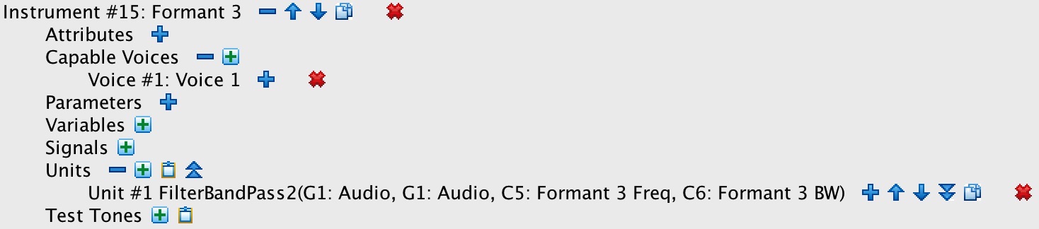
// Ins 15: Formant 3
note 15 1 15 0 0.25 2.00
// Ins 5: EnvSust
note 16 1 5 0 0.25 2.25 5000 0.03 0.1
// Ins 21: Rebalance-Output
note 17 1 21 0 0.25 2.00
end 2.50
ToneClusterOrch.xml.
The Sound orchestra used to generate sound examples for this fourth exercise is outlined in
Figure 5-1, while Listing 2 shows how this orchestra
would be used to synthesize a diphthong transitioning from the neutral vowel ə
to the long-E sound i.
This second orchestra carries over all of the waveforms listed
in the earlier ToneClusterOrch.xml (Figure 1-1); however the waveforms of particular interest
to the present exercise are:
- Waveform #916: Octave 16 used to source from Closed Octave-Doubled Clusters.
- Waveform #47: Muted Octave 16 used to source from Closed ‘Pink’ Clusters.
- Waveform #1: Sine used to source from Open Clusters.
Of the voice-scoped signals, G1 has been retained
for audio data, G2 has
been re-purposed for envelope control, and G3 has been dropped.
Instrument #1: Tone has been retained for tone generation, Instrument #5: EnvSust has been retained to generate an envelope,
and Instrument #21: Rebalance-Output carries over to normalize the audio content, to impose the envelope from Instrument #5: EnvSust,
and to mix the completed sound into the file-output buffer for channel #0.
What's new among the voiced-scoped entities in TriplePoleOrch.xml (Figure 5-1)
are six contours. There are two contours for each of the three cascaded band-pass
filters, one contour to control the filter's peak frequency and a second contour to control the bandwidth.
All six of these contours employ a spline-exponential interpolating mode.
Exponential interpolation is suitable for frequencies since values change by equal ratios
over equal increments of time.
Imposing a spline condition upon the interpolation
means that values change very slowly at the starting and ending portions of the segment; change is concentrated at
the middle portion of the segment.
Also new to TriplePoleOrch.xml are three new instruments which impose band-pass filtering and which
link their filter arguments directly to the six contours just described:
-
Instrument #13: Formant 1 implements a band-pass filter which produces the lower of the three spectral peaks.
It draws its center frequency from C1: Formant 1 Freq
and its bandwidth from C2: Formant 1 BW.
Instrument #13: Formant 1 employs a Butterworth band-pass algorithm; this
kind of filter is nicely symmetric and does a particularly good job at suppressing frequencies on both sides of the pass-through band.
Activating Instrument #13: Formant 1 requires seven statements in Listing 2:
-
Three
rampstatements describe how C1: Formant 1 Freq evolves over the 2.25-second duration of the note list: a 0.25-second segment holding steady at the origin frequency 414; a 2.0-second segment transitioning from frequency 414 to frequency 277; and a final 0.25-second segment holding steady at the goal frequency 277. -
Three additional
rampstatements describe how C2: Formant 1 BW evolves. In each case the bandwidth values are 20% of the corresponding frequency values. - Note statement #13 activates Instrument #13: Formant 1 (coincidence not intended) 0.25 seconds into the note list and sustains the invocation of Instrument #13: Formant 1 for 2.0 seconds.
-
Three
-
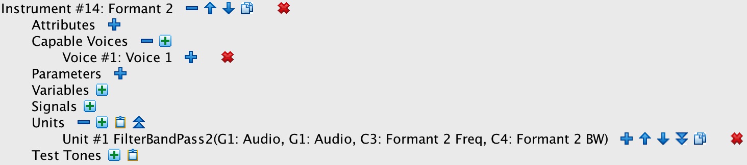
Instrument #14: Formant 2 implements a band-pass filter which produces the middle of the three spectral peaks.
It draws its center frequency from C3: Formant 2 Freq
and its bandwidth from C4: Formant 2 BW.
Instrument #14: Formant 2 employs MUSICV's original FLT algorithm, whose frequency
response differs from the Butterworth algorithm employed by Instrument #13: Formant 1. The FLT response is characterized by substantial bleed-through
of frequencies on the lower side of the pass-through band. Such bleed-through, which might be considered a defect
under other circumstances, is here considered an advantage.
Activating Instrument #14: Formant 2 requires seven statements in Listing 2:
-
Three
rampstatements describe how C3: Formant 2 Freq evolves over time: a 0.25-second segment holding steady at the origin frequency 2065; a 2.0-second segment transitioning from frequency 2065 to frequency 2208; and a final 0.25-second segment holding steady at the goal frequency 2208. -
Three additional
rampstatements describe how C4: Formant 2 BW evolves. In each case the bandwidth values are 10% of the corresponding frequency values. - Note statement #14 activates Instrument #14: Formant 2 0.25 seconds into the note list and sustains the invocation of Instrument #14: Formant 2 for 2.0 seconds.
-
Three
-
Instrument #15: Formant 3 implements a band-pass filter which produces the upper of the three spectral peaks.
It draws its center frequency from C5: Formant 3 Freq
and its bandwidth from C6: Formant 3 BW.
Like Instrument #14: Formant 2, Instrument #15: Formant 3 employs the FLT algorithm.
Activating Instrument #15: Formant 3 requires seven statements in Listing 2:
-
Three
rampstatements describe how C5: Formant 3 Freq evolves over time: a 0.25-second segment holding steady at the origin frequency 2570; a 2.0-second segment transitioning from frequency 2570 to frequency 3079; and a final 0.25-second segment holding steady at the goal frequency 3079. -
Three additional
rampstatements describe how C6: Formant 3 BW evolves. In each case the bandwidth values are 5% of the corresponding frequency values. - Note statement #15 activates Instrument #15: Formant 3 0.25 seconds into the note list and sustains the invocation of Instrument #15: Formant 3 for 2.0 seconds.
-
Three
Understand that no advantage was gained by implementing each formant filter as a separate instrument. The advantage offered
by voice scoping is the ability to swap elements in and out dynamically; e.g., to generate some sounds with three formants,
other sounds with two formants, and still other sounds with six formants. This does not happen in the present exercise.
Thus some notelist-coding efficiency could have been gained by consolidating all three filters into one instrument. The
number of note statements could have been reduced slightly,
although the number of ramp statements would have stayed the same.
Note-List Generation
The new presence of ramp statements imposed additional burdens
upon my notelist-generating program. I now needed efficient ways to request:
- “Generate a block of steady-state ramp statements which start at such-and-such a time, which hold for such-and such a duration, and which maintain values for these six contours”, or
- “Generate a block of transitional ramp statements which start at such-and-such a time, which unfold for such-and such a duration, and which prescribe origin and goal values for these six contours”.
This meant first making the InstrumentStack aware of all six contours defined for Voice #1 in
TriplePoleOrch. It meant next implementing a StackContourArray entity which belongs to the stack
and which encapsulates all the frequencies and bandwidths necessary to form a particular vowel. The StackContourArray
class in turn encloses a collection of StackContourValue instances, each of which stores a contour value and a reference
to the pertaining contour. For example, the neutral vowel ə would be described
by a StackContourArray enclosing six StackContourValue instances:
- The frequency 277 Hz. maps to contour C1: Formant 1 Freq,
- The bandwidth 277×20%=55 Hz. Hz. maps to contour C2: Formant 1 BW,
- The frequency 2208 Hz. maps to contour C3: Formant 2 Freq,
- The bandwidth 2208×10%=221 Hz. maps to contour C4: Formant 2 BW,
- The frequency 3079 Hz. Hz. maps to contour C5: Formant 3 Freq, and
- The bandwidth 3079×5%=185 Hz. maps to contour C6: Formant 3 BW.
Here the three formant values were obtained from a table of vowel formants, while the three bandwidth values were calculated according to a policy.
Given such vowel-describing entities, the InstrumentStack mandates two methods:
-
Method
createSteadyRampsgenerates steady-state ramps; it requires a notelist reference, a start time, a duration, and one vowel-entity reference. -
Method
createTransitionRampsgenerates transitional ramps; it requires a notelist reference, a start time, a duration, an origin-vowel reference, and a goal-vowel reference.
Efficient enough.
Sourcing from Closed Octave-Doubled Clusters
Now that we know both how the orchestra is designed and how the notelist-generating program functions, it's time to hear how well the new subtractive component enriches the diversity of clustered sounds. For this fifth exercise the source clusters are limited to semitones (12 per octave) and quarter-tones (24 per octave). The waveform employed for tones is consistently the octave-doubled type with equal amplitudes for harmonics #1, #2, #4, #8, and #16. The combined result gives the acoustic characteristics of White Noise.
The pair of sound examples displayed in Video 3-1a and Video 3-1b
effects a diphthong sourcing from an octave-doubled sine cluster.
The origin is the neutral vowel ə with formants at
277 Hz., 2208 Hz., and 3079 Hz.
The goal is the long-E sound i with formants at
414 Hz., 1516 Hz., and 2500 Hz.
The sound example displayed in Video 3-1c effects the same diphthong sourcing from an arpeggiated
quarter-tone cluster.
The pair of sound examples displayed in Video 3-2a and Video 3-2b subjects an octave-doubled sine cluster to filtering using the long-E formants at 414 Hz., 1516 Hz., and 2500 Hz. The sound example displayed in Video 3-2c effects the same vowel sourcing from an arpeggiated quarter-tone cluster.
The pair of sound examples displayed in Video 3-3a and Video 3-3b
effects a diphthong sourcing from an octave-doubled sine cluster.
The origin is a (as in father) with formants at
formants at 800 Hz., 1228 Hz., and 2500 Hz.
The goal is the long-E sound with formants at
414 Hz., 1516 Hz., and 2500 Hz.
The sound example displayed in Video 3-3c effects the same diphthong sourcing from an arpeggiated
quarter-tone cluster.
The pair of sound examples displayed in Video 3-4a and Video 3-4b
subjects an octave-doubled sine cluster to filtering using the long-O sound
o with formants at
414 Hz., 721 Hz., and 2406 Hz.
The sound example displayed in Video 3-4c effects the same vowel sourcing from an arpeggiated
quarter-tone cluster.
The pair of sound examples displayed in Video 835a and Video 3-5b
effects a diphthong sourcing from an octave-doubled sine cluster.
The origin is the long-E sound with formants at
277 Hz., 553 Hz., and 2420 Hz.
The goal is the long-U sound u with formants at
414 Hz., 1516 Hz., and 2500 Hz.
The sound example displayed in Video 3-5c effects the same diphthong sourcing from an arpeggiated
quarter-tone cluster.
The pair of sound examples displayed in Video 3-6a and Video 3-6b
effects a diphthong sourcing from an octave-doubled sine cluster.
The origin is a (as in father) with formants at
formants at 800 Hz., 1228 Hz., and 2500 Hz.
The goal is the rhotacized schwa sound ɚ (as in
better) with formants at 414 Hz., 1516 Hz., and 1800 Hz.
(Rhotacized schwa? That's not a vowel! No, but it's a liquid, and liquids are formed the same way vowels are formed.)
The sound example displayed in Video 3-6c effects the same diphthong sourcing from an arpeggiated
quarter-tone cluster.
Sourcing from Closed ‘Pink’ Clusters
All of the sound examples presented in Video 3-1a through Video 3-6b were sourced from octave-doubled clusters. While these examples confirmed that a great many differentiated sounds could be obtained, the extreme harshness of band-limited white noise penetrates through in every instance. The arpeggiated clusters presented in Video 3-1c through Video 3-6c are equally harsh. If I used such sounds in a composition, I would want to limit them to exceptional situations. For most of my sounds I would seek out something less abrasive. Now the discussion of Waveform Clusters suggested that if band-limited white noise wasn't appropriate, then perhaps using pink or brown sources might provide levels of mitigation. For example, Figure 3-5a and Figure 3-5b presented a tone-cluster realization of band-limited pink noise.
To hear what happens when a ‘pink’ quarter-tone cluster is filtered to effect a diphthong from the neutral vowel
ə to the long-E sound i,
click here. Compare this sound to the same diphthong sourced from a ‘white’
quarter-tone cluster in Video 3-1b.
The ‘pink’ sound is definitely less harsh although it retains much of the dirtiness3 associated with white noise. The ‘pink-sourced’ diphthong is also darker than the ‘white-sourced’ diphthong owing to the suppression of higher frequencies. It seems to me that suppressing these higher frequencies does not promise to be fruitful if we are at the same time expecting formants in the same frequency regions to develop the character of the sound.
Sourcing from Open Clusters
The vowel and diphthong sounds presented so far have sourced from closed cluster voicings. Now its time to hear what happens when the source is swapped over to open voicings. The next six sound examples do this. The change is not radical to my ear, but the open-voiced quarter tone sources seem to me less blaring than closed-voice semitone sources and less dirty than closed-voice quarter-tone sources.
Video 4-1: Open quarter-tone cluster filtered through
a/i diphthong.
Compare with Video 3-1b.
|
Video 4-2: Open quarter-tone cluster filtered through
i vowel.
Compare with Video 3-2b.
|
Video 4-3: Open quarter-tone cluster filtered through
ə/i diphthong.
Compare with Video 3-3b.
|
Video 4-4: Open quarter-tone cluster filtered through
o vowel.
Compare with Video 3-4b.
|
Video 4-5: Open quarter-tone cluster filtered through
i/u diphthong.
Compare with Video 3-5b.
|
Video 4-6: Open quarter-tone cluster filtered through
a/ɚ diphthong.
Compare with Video 3-6b.
|
Diversity of Vowel-Derived Sounds
The number of sounds available when combining three static formants is huge. Consider first the number vowels combined with the number of liquids.4 Beyond that, dynamic transitions from one set of formants to another are themselves recognized as phonemes, with further distinctions drawn by the rate of transition. Thus voiced plosive consonants employ transitions under 50 msec., glides employ transitions around 100 msec., and diphthongs employ transitions of 300 msec. or longer. Also, one must recognize that the tables of vowels and liquids presented on this site apply specifically to adult males. The simple process of transposition can derive new formant sets for women, for children, and for singing mice.
Static Antiformants
As an alternative to using band-pass filters to create spectral formants, this sixth exercise considers using band-reject
filters to create anti-formants, or troughs in the frequency spectrum. Anti-formants are associated with the
nasal consonants m (bilabial), n,
(alveolar) and ŋ (velar). Nasal sounds typically involve just one anti-formant.
However it is not the purpose of this exercise to reproduce nasal sounds. Rather the present purpose is to further mitigate the harshness of tone clusters through very aggressive processing using three anti-formants. The subtractive-synthesis design employed for the present exercise cascades three notch filters interleaved with three formant filters.
This is my third iteration at triple-antiformant filtering. The first iteration combined three notch filters with a single low-pass set around G8 (6272 Hz.). Left mostly to themselves in this manner, the notch filters completely blanked out frequencies in the lowest octaves of the cluster. The second iteration interleaved anti-formant, formant, anti-formant, formant, anti-formant, formant. Such interleaving greater purchase to the between-antiformant bands; however, the resulting spectra still contained preponderances of upper frequencies. This third iteration inserted a new formant between 0 Hz. and the first antiformant, dropped the formant above the third antiformant, and added a low-pass filter with its cutoff set to 6272 Hz. Although I preferred the results from the second iteration in some ways, this third set of sounds is dydactically more suitable because the antiformants clearly show up in the frequency-spectrum graphs.
The next question was where to locate the anti-formants. I decided to go for nine different filter configurations, which would be arbitrarily labeled using the upper-case letters A through I. Remember that the source spectrum ranges from G3 (196.0 Hz.) to G8 (6272 Hz.). I elected to establish three non-overlapping ranges:
- Lower anti-formants increase in whole-tone increments from A3 (220.0 Hz.) to C#5 (554.3 Hz.).
- Middle anti-formants increase in whole-tone increments from F5 (698.4 Hz.) to A6 (1760 Hz.).
- Upper anti-formants would increase in whole-tone increments from C#7 (2217 Hz.) to F8 (5587 Hz.).
From there, having no idea what sounds would result but wanting no specific antiformant setting to be shared between any two configurations, I let the computer subject each antiformant range to a random shuffle, then accepted the combinations that resulted.
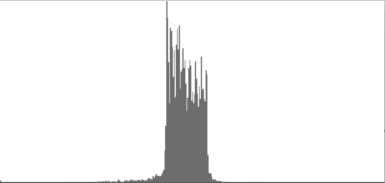
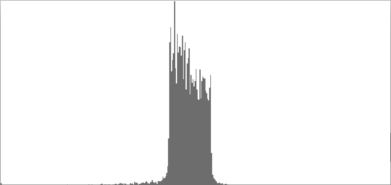
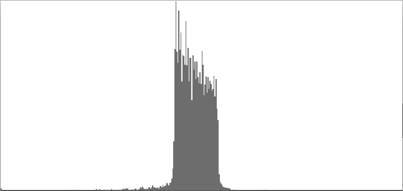
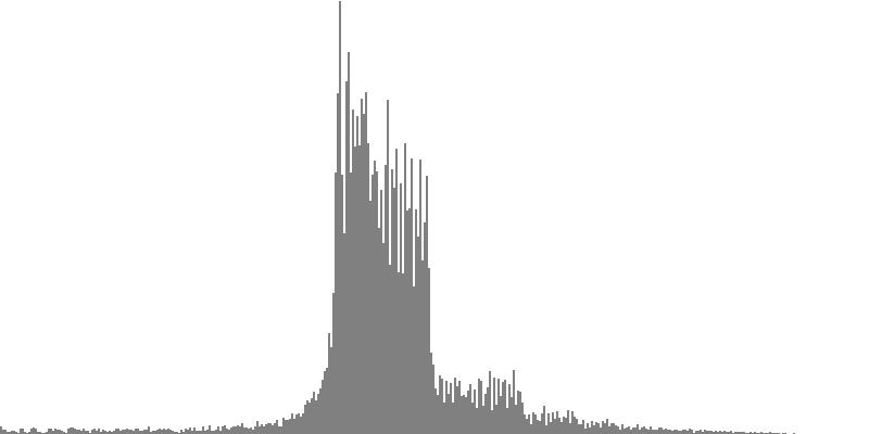
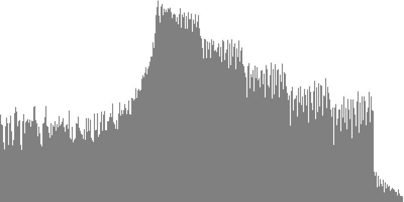
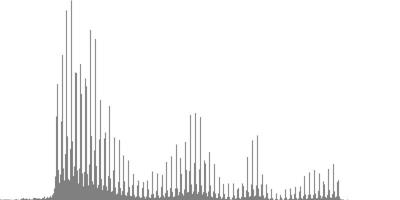
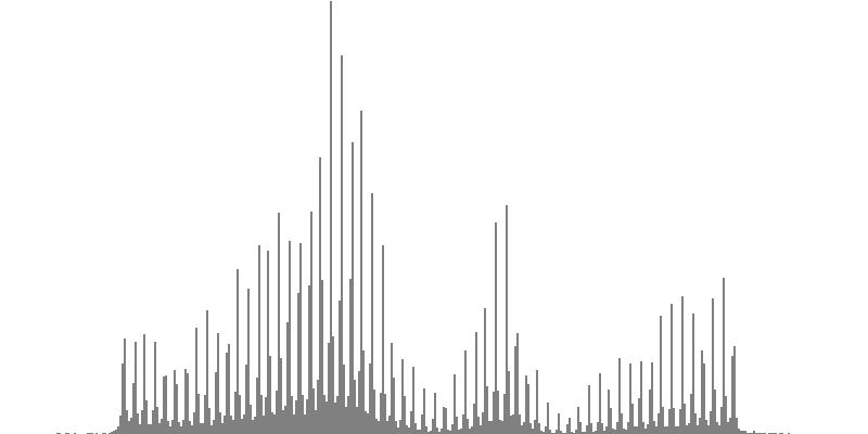
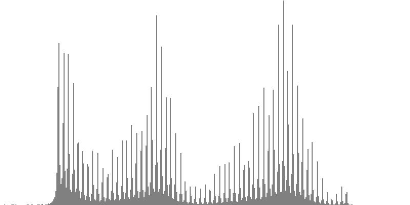
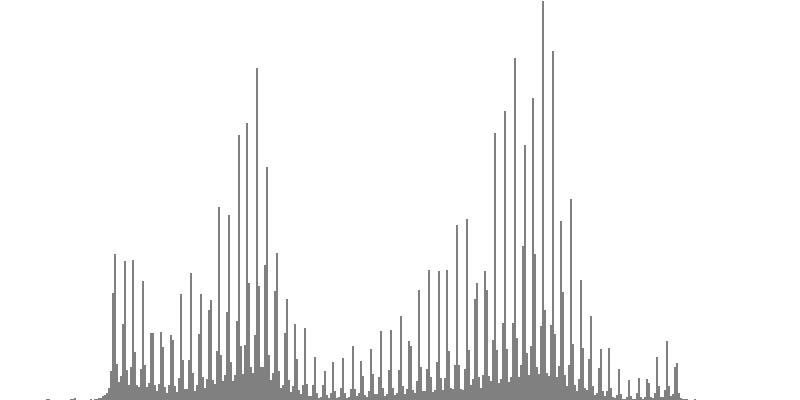
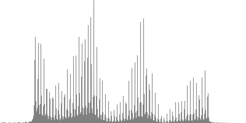
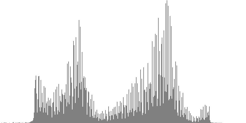
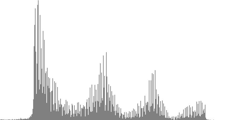
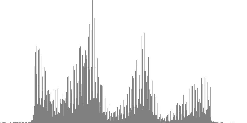
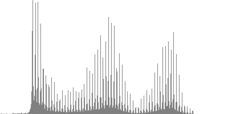
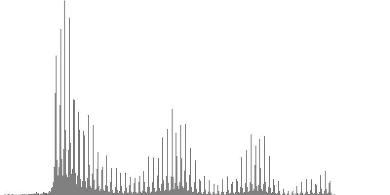
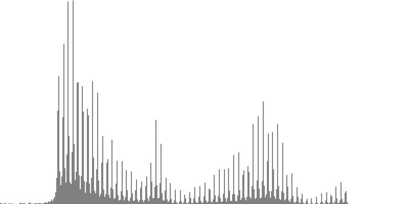
The graphs shown below plot cents on the horizontal axis against sample magnitudes on the vertical axis. The horizontal axis ranges from G2 (one octave below the cluster's lowest pitch) to G9 (one octave above the cluster's highest pitch). The vertical axis is scaled so that the tallest peak fills the entire vertical range.
|
|
|
||
| Figure 7-1a: The source is an octave-doubled sine cluster dividing the octave into 12 equal parts. This source is processed through Configuration A, with anti-formants at 554.3, 1568, and 2794 Hz. To hear a realization, click here. | Figure 7-2a: The source is an octave-doubled sine cluster dividing the octave into 12 equal parts. This source is processed through Configuration B, with anti-formants at 220.0, 1109, and 2217 Hz. To hear a realization, click here. | Figure 7-3a: The source is an octave-doubled sine cluster dividing the octave into 12 equal parts. This source is processed through Configuration C, with anti-formants at 311.1, 987.7, and 4978 Hz. To hear a realization, click here. | ||
|
|
|
||
| Figure 7-1b: The source is an octave-doubled sine cluster dividing the octave into 24 equal parts. This source is processed through Configuration A, with anti-formants at 554.3, 1568, and 2794 Hz. To hear a realization, click here. | Figure 7-2b: The source is an octave-doubled sine cluster dividing the octave into 24 equal parts. This source is processed through Configuration B, with anti-formants at 220.0, 1109, and 2217 Hz. To hear a realization, click here. | Figure 7-3b: The source is an octave-doubled sine cluster dividing the octave into 24 equal parts. This source is processed through Configuration C, with anti-formants at 311.1, 987.7, and 4978 Hz. To hear a realization, click here. | ||
|
|
|
||
| Figure 7-4a: The source is an octave-doubled sine cluster dividing the octave into 12 equal parts. This source is processed through Configuration D, with anti-formants at 246.9, 698.4, and 4434 Hz. To hear a realization, click here. | Figure 7-5a: The source is an octave-doubled sine cluster dividing the octave into 12 equal parts. This source is processed through Configuration E, with anti-formants at 392.0, 1244, and 3136 Hz. To hear a realization, click here. | Figure 7-6a: The source is an octave-doubled sine cluster dividing the octave into 12 equal parts. This source is processed through Configuration F, with anti-formants at 277.2, 879.9, and 2489 Hz. To hear a realization, click here. | ||
|
|
|
||
| Figure 7-4b: The source is an octave-doubled sine cluster dividing the octave into 24 equal parts. This source is processed through Configuration D, with anti-formants at 246.9, 698.4, and 4434 Hz. To hear a realization, click here. | Figure 7-5b: The source is an octave-doubled sine cluster dividing the octave into 24 equal parts. This source is processed through Configuration E, with anti-formants at 392.0, 1244, and 3136 Hz. To hear a realization, click here. | Figure 7-6b: The source is an octave-doubled sine cluster dividing the octave into 24 equal parts. This source is processed through Configuration F, with anti-formants at 277.2, 879.9, and 2489 Hz. To hear a realization, click here. | ||
|
|
|
||
| Figure 7-7a: The source is an octave-doubled sine cluster dividing the octave into 12 equal parts. This source is processed through Configuration G, with anti-formants at 349.2, 1760, and 5587 Hz. To hear a realization, click here. | Figure 7-8a: The source is an octave-doubled sine cluster dividing the octave into 12 equal parts. This source is processed through Configuration H, with anti-formants at 440.0, 1397, and 3520 Hz. To hear a realization, click here. | Figure 7-9a: The source is an octave-doubled sine cluster dividing the octave into 12 equal parts. This source is processed through Configuration H, with anti-formants at 493.8, 783.9, and 3951 Hz. To hear a realization, click here. | ||
|
|
|
||
| Figure 7-7b: The source is an octave-doubled sine cluster dividing the octave into 24 equal parts. This source is processed through Configuration G, with anti-formants at 349.2, 1760, and 5587 Hz. To hear a realization, click here. | Figure 7-8b: The source is an octave-doubled sine cluster dividing the octave into 24 equal parts. This source is processed through Configuration H, with anti-formants at 440.0, 1397, and 3520 Hz. To hear a realization, click here. | Figure 7-9b: The source is an octave-doubled sine cluster dividing the octave into 24 equal parts. This source is processed through Configuration I, with anti-formants at 493.8, 783.9, and 3951 Hz. To hear a realization, click here. |
Moving Antiformants
Closed and Arpeggiated Clusters; Rates of Transition
This seventh exercise juggles four of the filter configurations developed in the just completed section on Static Antiformants:
- Configuration A has zeros at 554.3, 1568, and 2794 Hz.
- Configuration B has zeros at 220.0, 1109, and 2217 Hz.
- Configuration C has zeros at 311.1, 987.7, and 4978 Hz.
- Configuration D has zeros at 246.9, 698.4, and 4434 Hz.
The sequence of A's, B's, C's, and D's was generated using statistical feedback with equal weight to each of these three configurations and subject to the constraint of no configuration directly succeeding itself. The same sequence of filter configurations is employed in all ten sound examples.
There are two points of interest in this seventh exercise. One point of interest is how the results are affected by source. The other point of interest is the rate of transition.
- The component tones in each of Video 5-1a through Video 5-5b are sine tones doubled at the 2nd, 4th, 8th, and 16th harmonic. The sources for the (a) examples are sustained block clusters. For the (b) examples I have broken out the source clusters using the method described previously for Arpeggiated Clusters.
-
Each example begins with a quarter second of silence, presents five seconds of sound, then ends with an additional quarter second of silence.
The five seconds of sound divide into moments lasting 0.125 seconds each. Each moment consists of a transition phase and a steady-state phase.
Within the transition phase, transitions between configurations are effected using spline-exponential interpolations for
each filter frequency and for each filter bandwidth. Transition times descend in reverse Fibonacci order:
- 80 msec. in Video 5-1a and Video 5-1b,
- 50 msec. in Video 5-2a and Video 5-1b,
- 30 msec. in Video 5-3a and Video 5-3b,
- 20 msec. in Video 5-4a and Video 5-4b,
- 10 msec. in Video 5-5a and Video v-5b.
Open Clusters; Mixed Articulation
The sound examples presented as Video 5-1a through Video 5-5b explored triple-antiformant filtering applied to two quarter-tone cluster sources: static closed (Video 5-1a through Video 5-5a) and arpeggiated, which are also closed (Video 5-1b through Video 5-5b). It still remains to demonstrate what happens when the source is an open cluster.
The example presented in Video 6 begins with a quarter second of silence, presents eight seconds of sound, then ends with an additional quarter second of silence. The eight seconds of sound divide into 64 moments lasting 0.125 seconds each. All moments divide into transition phase and steady-state phases. Some moments are preceded by silences whose time is appropriated from the previous moment's steady-state phase.
Having made the point that rapid transition times produce a more clearly articulated effect that slower transition times, I decided for this eighth exercise to mix transitions up and to limit the transition intervals to two: 20 msec. for the rapid case and 80 msec. for the slower case. Going forward for this exercise, the term sustained will refer to 20 msec. transitions while the term slurred will refer to 80 msec. transitions. Both types of articulation should be understood to happen under a sustained envelope.
I also thought to enrich this exercise with a third detached articulation, which I thought would be more emphatic than than sustained or slurred. This third type of articulation also employs rapid transition intervals; however it employs three additional features:
- First, detached articulations are preceded by silences. The duration of silence, based on experience working with articulative silences, is set to 80 msec.
- Second, the new envelope initiated by a detached articulation rises very rapidly from zero to full amplitude. This rise time, based on comparisons undertaken for attack durations, is set to 10 msec.
-
Third, the steady-state timbre (read: filter configuration) is approached from somewhere different than the preceding steady
state (before the silence). Consider the example of moments #8, #9, #10, #11 the sequence of steady-state timbres is
H, I, F, F.
- The articulation for moment #9 is sustained, so the first phase of moment #9 transitions over 20 msec. from H (the steady-state timbre of moment #8) to I (the steady-state timbre of moment #9).
- The articulation for moment #10 is slurred, so the first phase of moment #10 transitions over 80 msec. from I (the steady-state timbre of moment #9) to F (the steady-state timbre of moment #10).
- The articulation for moment #11 is detached, so by contrast the timbre at the beginning of moment #11's transition phase may not carry over H from moment #10. Rather, moment #11 begins with timbre H, transitions over 20 msec. to F, which latter holds through.
Generating the notes for this example thus came down first to deciding how each moment should be articulated and second to deciding which timbres should be employed for which moments. Statistical feedback drove each set of decisions:
- The selected sequence of articulations is presented in the middle row of Table 1. Here bullets (•) indicate detached articulations, which have a weighting factor of 3/13. Greater-than signs (>) indicate sustained articulations, which have a weighting factor of 4/13. Tildes (~) indicate slurred articulations, which have a weighting factor of 6/13. All positions are stressed equally and the heterogeneity value is 0.1. The constraints are these: The initial and final articulations must be detached. Detached articulations must be lead or followed by slurs. Likewise, sustained articulations must be lead or followed by slurs.
- The selected sequence of timbres is presented in the bottom row of Table 1 using the designations F, G, H, I. Each of the four timbre options has equal weight. Positions are equally stressed, though it probably would have been better to assign lighter stress to opening timbres for detached moments. There is just one constraint: no timbre may succeed itself.
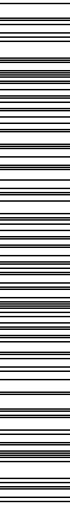
Video 6: Open cluster with 3 levels of articulation.
Listening to Video 6 uncovers an unintended consequence. Sustained articulations transitioning into the timbre G are much more emphatic than articulations transitioning into any other timbre. The effect is not disturbing but it makes a hash out of the accentuation sequence presented in the middle row of Table 1.
Comments
- Waveform #1 always indicates a sine wave in a Sound orchestra.
- The fair-share principle generalizes the equal-emphasis principle to non-uniform weights.
- The word dirty has a long association with noise. My mentor Lejaren Hiller once commented that back in the analog days of electronic music, he and his contemporaries used to generate noise by “sampling a dirty transistor”.
- I have no idea how many distinct vowel-like sounds are neglected by the International Phonetic Alphabet, but one can reasonably assume that if a sound is formable by human lips and tongue, then there is at least one of the Earth's six thousand languages that makes use of it.
Next topic: Open Quarter-Tone Clusters
| © Charles Ames | Page created: 2017-08-15 | Last updated: 2017-08-15 |