Synthesizing Noise Sounds
Overview
This page explains how digital synthesis engines generate noise. It also demonstrates how noise spectra can be shaped by digital filtering. To benefit from this page you should already understand how instruments are built up from units (if not see Implementing a Sound-Synthesis Instrument), and you should also understand the components of a note list (if not see Note-List Instructions).
Several of the activities on this page employ processes of equalization to conform the digital noise generator's non-uniform frequency spectrum to various profiles. The term ‘equalization’ refers to separating a source sound apart into frequency bands and then remixing these bands to obtain a desired overall frequency profile. Although the term literally suggests that this profile be flat, in practice equalization can be used to shape an input spectrum in a variety of ways. Balance need not be uniform!
A frequency-spectrum graph plots amplitude on the vertical scale against frequency on the horizontal scale. To that extent frequency-spectrum graphs resemble the frequency-response graphs used to analyze filter banks on the Digital Filtering pages. The difference is how the graphs are obtained:
- In the frequency-response graphs shown elsewhere, the value for a particular frequency is obtained by measuring the signal strength produced when a filter bank is excited by a sine wave of that frequency.
- In the frequency-spectrum graphs shown on this page, the value for a particular frequency is obtained by measuring the signal strength produced by subjecting a sound source to narrow band-pass filtering centered at the indicated frequency.
The horizontal (frequency) scale of a frequency-spectrum graph can be either linear or logarithmic:
- When the frequency scale is linear, values are measured in Hertz (abbreviated Hz.) — that is, in cycles per second. The width of a region in the lower (leftward) portion of the graph represents the same difference in cycles per second as the width of an equal-sized region in the upper (rightward) portion of the graph. This is not how our ears perceive frequency differences. For example, there is a difference of about two cycles per second between C1 (32.70 Hz.) and C#1 (34.65 Hz.), which we hear as a semitone. However the difference between C4 (261.6 Hz.) and C#4 (277.2 Hz.) is about 16 cycles per second, yet we also hear this interval as a semitone.
- When the frequency scale is logarithmic, values are measured in cents — that is, in hundredths of a semitone. The width of a region in the lower (leftward) portion of the graph represents the same difference in cents as the width of an equal-sized region in the upper (rightward) portion of the graph. And a semitone has the same width anywhere along the frequency axis.
Likewise, the vertical (amplitude) scale of a frequency-spectrum graph can be either linear or logarithmic:
- When the amplitude scale is linear, values are measured in sample magnitudes. The width of a region in the lower (leftward) portion of the graph represents the same sample-magnitude difference as the width of an equal-sized region in the upper (rightward) portion of the graph. This is not how our ears perceive amplitude differences.
- When the amplitude scale is logarithmic, values are measured in decibels. The width of a region in the lower (leftward) portion of the graph represents the same difference in decibels as the width of an equal-sized region in the upper (rightward) portion of the graph. In particular, the difference between two adjacent dynamic levels (e.g. mp and mf) is 4-6 decibels. The MIDI velocity scale, which ranges from 0 to 127, is also an example of a logarithmic amplitude scale with increments of about 16 between dynamic levels.
Since logarithmic scales best represent how the ear perceives both frequencies and amplitudes, it follows logically that log/log plots (also known as Bode plots) are the most ‘natural’ way to present frequency spectra. However such is not typically the case in practice. Although log/log plots are used in discussions of colored noise, it is much more common to plot frequencies linearly.
The frequency-spectrum graphs shown on this page were generated using the Wave-File Viewer. The instrument stack described under the next heading was used to generate a single monaural sound, which was saved as a wave file. This wave file was then loaded into the Wave-File Viewer, and spectral graphs were obtained following the procedures described in the Wave-Viewer Instructions.
Orchestra
NoiseOrch.xml implements a Sound orchestra which
has been designed specifically to accompany this page.
Sound examples for the current page are provided in the form of note lists referencing this orchestra.
Audio realizations are provided for each note list.1
The text following provides a broad overview of NoiseOrch.xml and also many details.
NoiseOrch.xml actually defines a single ‘stack’ of instruments (alternatively, a ‘meta-instrument’).
The stack has four categories of swappable component.
It takes several notes to make a sound using this stack:
- One or more notes to generate a “source” sound. A sound will normally have one source but chords are also possible. The “source” category of instruments has five members:
- Instrument #1: Classic Noise
- Instrument #2: Balanced-Bit Noise
- Instrument #3: Buzz
- Instrument #4: Modulated Sine
- Instrument #5: Percussive Noise
- Zero or one note to capture the source signal's RMS power envelope. The “source-power extraction” category of instruments contains just one member: Instrument #10: RMS. The power-envelope note may be omitted only if no filtering operations follow.
- Zero or more notes to modify the sound using filtering operations. The modifier notes can employ any combination of instruments in the “signal-modifying” category, and combinations may use the same instrument more than once. The “signal-modifying” category of instruments has five members:
- Instrument #11: Low Pass
- Instrument #12: High Pass
- Instrument #13: Band Pass BW
- Instrument #14: Band Pass FLT
- Instrument #15: Band Reject
- Instrument #16: Sine Wave Modulator
- Instrument #17: Linear Equalizer
- Instrument #18: Logarithmic Equalizer
- Exactly one note to rebalance the sound and output it to channel 0. The “rebalancing/output” category of instruments contains two members, of which one must be chosen:
- Instrument #21: Rebalance-Output is employed when Instrument #10: RMS is also present.
- Instrument #22: Output is employed when Instrument #10: RMS is not present.
Figures 1 (a) through 4 (b) provide flow diagrams for each category (a) along with an image of one member instrument (b). You should understand a couple of points about the flow diagrams (a):
- First point: Where the flow of signals extends outside the dashed rectangles, the signals are associated with the voice rather than the instrument.
- Second point: Voice-level signals always initialize to zero (unlike instrument-level signals which must be explicitly initialized).
- Third point: During audio-rate calculations, the Sound engine processes notes in voice-id order, and when voice id's are the same, in note-id order.
NoiseOrch.xml imposes a restriction on how notes align, which is that start times and durations must be identical for the
“source-power extraction”, “signal-modifying”, and “rebalancing/output” phases. You ignore
this restriction on pain of generating very unpleasant pops. “Source” notes may not extend outside the overall time interval.
Within this time interval “source” notes can occur sequentially or simultaneously; there can also be silences between
“source” notes.
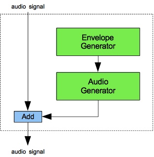
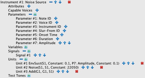
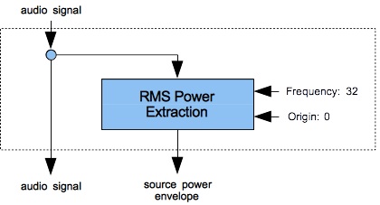
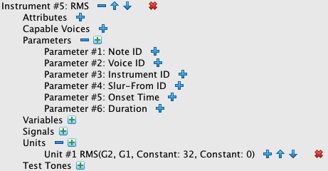
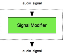
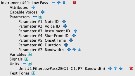
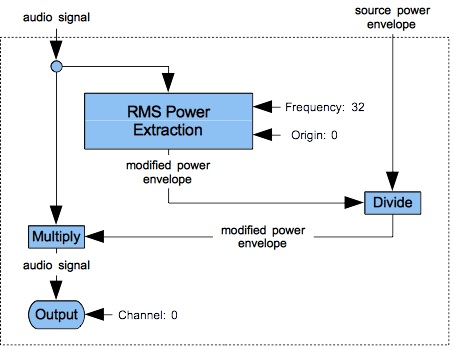
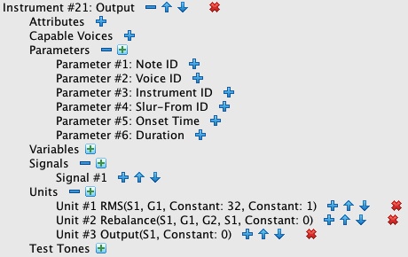
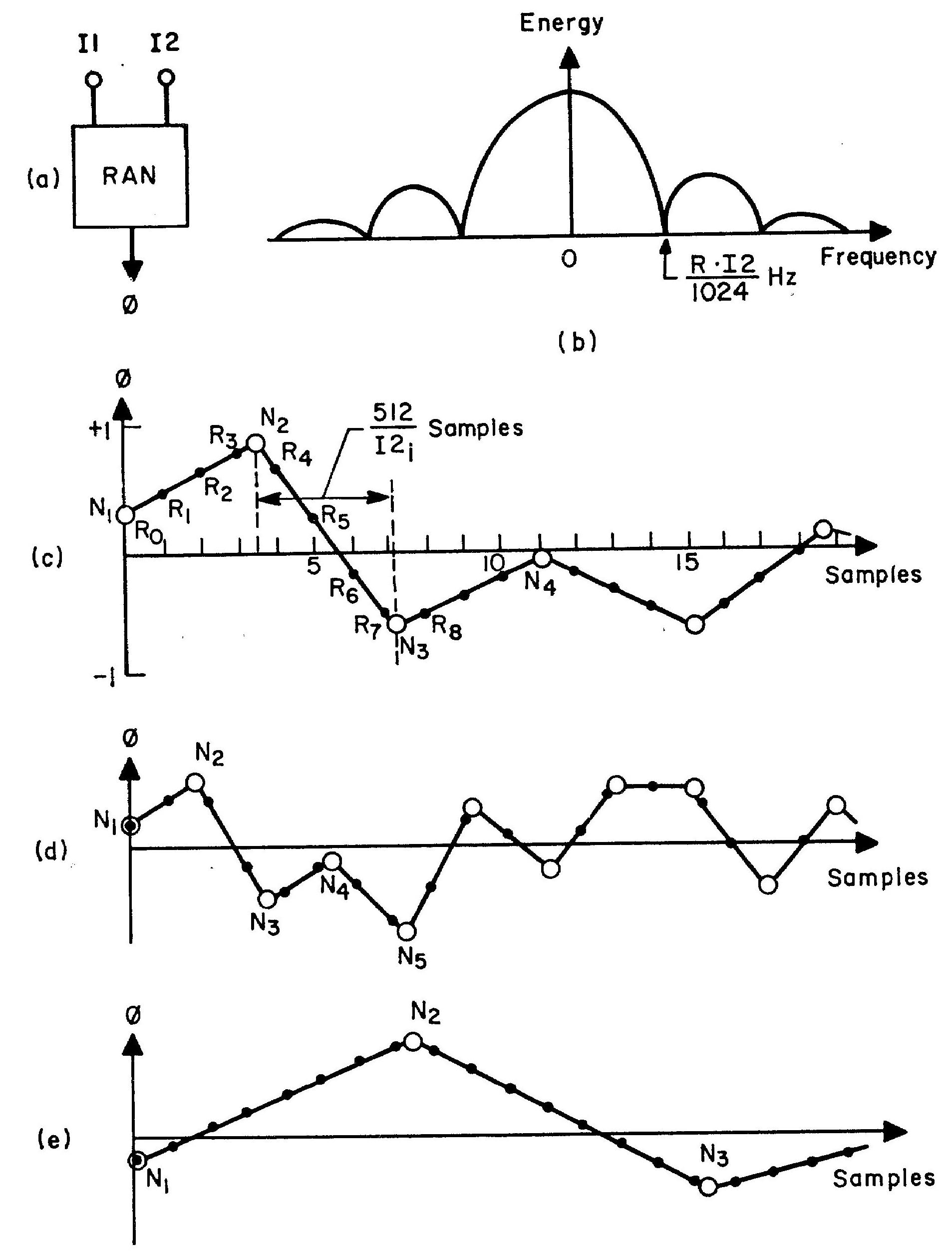
Figure 5: Random generator — RAN: (a) block diagram; (b) output spectrum; (c) medium-frequency random function, (d) high-frequency random function, (e) low-frequency random function. Source: The Technology of Computer Music, p. 69 (originally figure 36).
How Computers Generate Noise
My Sound engine's Noise unit implements MUSIC-V's “Random Function Generator”
(RAN) as described on pages 128-129 of The Technology of Computer Music.
The original diagram illustrating how this unit operates is reproduced in Figure 5.
Every K samples, this unit calls the classic random number generator
to select a value ranging uniformly from -1 to +1.
The unit then interpolates linearly between consecutive samples.
The selection interval K is calculated by dividing the sample rate by the frequency of selection.
Input I1 is an amplitude used to scale the interpolated values.
Input I2 is an artifact of the RAN unit's implementation. The value 512 is an arbitrary time-scaling factor.
Instead of expecting the frequency of selection directly, I2 expects the ratio of the selection frequency to the
sample rate.
Video 1-1 and Video 1-2 animate the selection process diagrammed statically in Figure (c). For both animations the sampling rate is one sample per pixel, so the points R0, R1, R3, … cluster together without intervening time. The process cascades two stages. The left-side stage labeled Noise is a sample generator which produces a new sample during each frame of the animation (25 frames per second). The right-side stage labeled Output is a signal queue. Each frame scrolls the contents of the Output rightwards by one pixel, allowing the newly generated sample to be plotted in the leftmost position. The samples thus plotted proceed from newer samples on the left to older samples on the right, reversing theorder of presentation normally expected a time-series graph.
Watch what happens within the noise generator. The position 10 pixels in from the leftward border represents the current moment. Sample selection is depicted by a vertical line which extends from the x-axis to the current value and a horizontal arrow showing where this value will be plotted in the output queue. Values between the generator's left border and the current position are past history — these are not actually retained by the noise generator. Values to the right of the current position show the current trend (the slope) and the number of samples remaining in the current segment. Understand that the generator holds no information other than the current value, the slope, and the remaining segment length. Each new frame of the animation decreases the number of samples remaining by 1. When this number drops to zero, the noise generator initiates a new segment and asks the random number generator what value should be targeted during the new segment.
Video 1-1: Noise generation with a reselection rate of 30 samples/segment.
Video 1-2: Noise generation with a reselection rate of 15 samples/segment.
One issue when using noise as a sound source is rumble, which is the tendency of a noise to vary in amplitude. One method of suppressing rumble is to normalize the Noise output. That is, you extract the RMS power envelope from a Noise signal using the RMS unit, then divide the same Noise signal by the power envelope.
Listing 1 (a): Noise generated using the Noise unit with the cutoff frequency set to 3333 (one-third of the Nyquist limit). To hear a realization, click here.
Of special interest in Figure 5 is item (b), which plots the noise generator's frequency spectrum. The graph is confusing because it plots both positive and negative frequencies. However since the graph is symmetrical around the zero point and, since a negative-frequency sine wave equals a positive-frequency sine wave phase-shifted by 180°, and since the human ear does not perceive phase, you can simply ignore the left half of the graph.
The note list presented in Listing 1 (a) generates noise with a cutoff frequency of 3333 Hz. lasting for four seconds.
You must substitute your own working directory in the orch statement.
Having no “signal-modifying” phase means that the “source power envelope” and “modified power envelope”
will be identical. Thus it is not necessary to extract the power envelope using Instrument #10: RMS and to
rebalance the signal using Instrument #21: Rebalance-Output.
Instead the results from Instrument #1: Classic noise are written out directly using Instrument #22: Output.
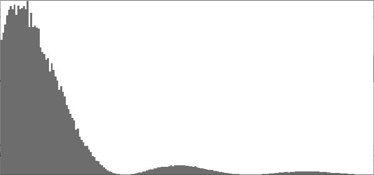
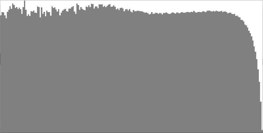
Figure 6: Linear/linear plot of frequency spectrum produced by the Noise unit with the cutoff frequency set to 3333 (one-third of the Nyquist limit).
Figure 6 presents a frequency-spectrum graph of the sound generated using Listing 1 (a), which
saves to the filename NoiseClassic.wav.
Notice that the first time the graph dips to zero corresponds to the cutoff frequency of 3333 Hz. I cannot explain the small differences
in shape between Figure 6 and Figure 5 (b) because I do not know how the authors of
The Technology of Computer Music obtained their graph.
Listing 1 (b) generates classic noise at a CD-audio sample rate (44100 Hz.) and Nyquist cutoff frequency (22050 Hz.),
saving the result to a file named NoiseClassic2.wav.
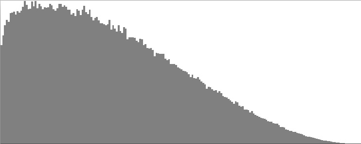
Figures 7 (a-c) give linear/linear (a), linear/logarithmic
(b), and Bode plots (c), of the spectrum produced by Listing 1 (b).
The Bode plot in Figure 7 (c) averages around -7 dB up through around C5 (an octave above middle C), slopes upward gradually
to around -1 dB around C9 (one octave higher than the highest C on a piano), then drops away precipitously as pitch values move into the
inaudible range. Favoring the higher registers in this manner puts the spectrum on the blue side of white noise, an example
of which may be found at www.audiocheck.net.
The section below on Colored Noise explains how output from the Noise unit
can be actively reshaped to conform to prescribed colors.
|

|
|
| Figure 7 (a): Linear/linear plot of frequency spectrum produced by Listing 1 (b). | Figure 7 (b): Linear/logarithmic plot of frequency spectrum produced by Listing 1 (b). | Figure 7 (c): Bode plot of frequency spectrum produced by Listing 1 (b). |
Balanced-Bit Noise
My Balanced Bit Generator is described on this site in the pages devoted to Drivers and Transforms. My Sound engine's NoiseB unit works like MUSIC-V's “Random Function Generator” except that wherever the classic unit calls upon the standard random-number generator, the NoiseB unit calls upon a balanced-bit driver.
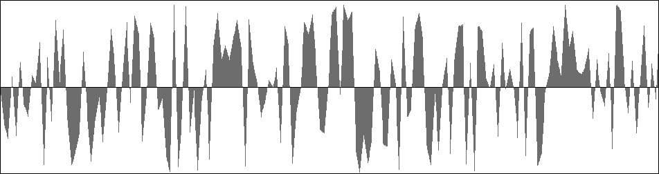
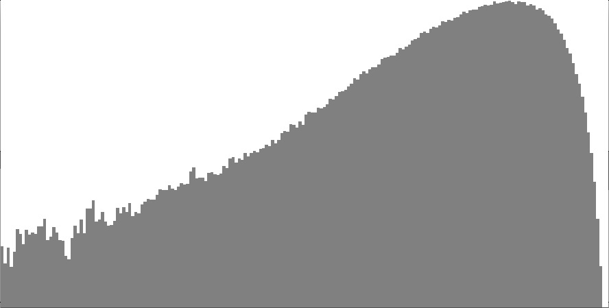
Figure 8 (a): Excerpt of wavefile produced by the Noise unit with the cutoff frequency set to 3333 (one-third of the Nyquist limit).
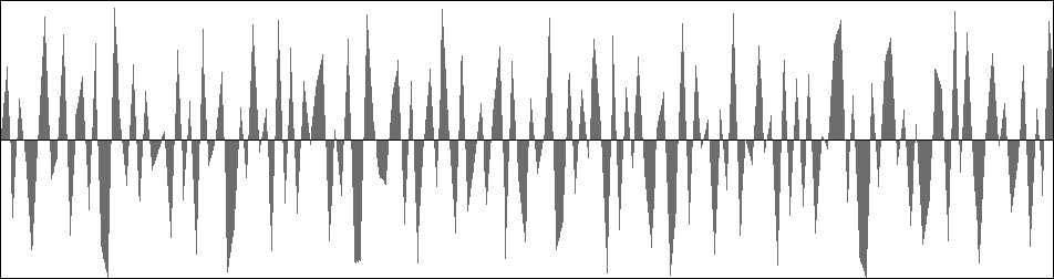
Figure 8 (b): Frequency spectrum produced by the NoiseB unit with the cutoff frequency set to 3333 (one-third of the Nyquist limit).
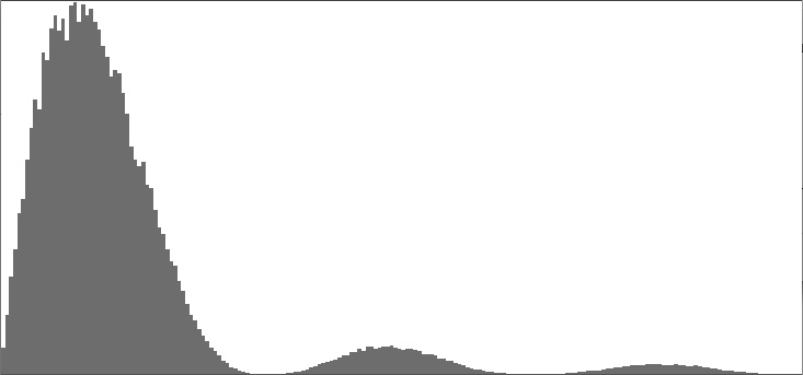
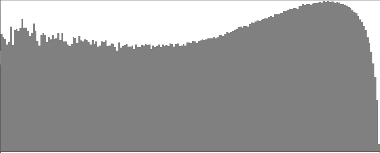
Figure 9: Frequency spectrum produced by the NoiseB unit with the cutoff frequency set to 3333 (one-third of the Nyquist limit).
Output from the Noise unit and NoiseB units are presented side-by-side in Figure 8 (a) and Figure 8 (b). The difference between the two graphs is that Figure 8 (a) tends to linger on one side or the other of the zero line while Figure 8 (b) distributes goal points uniformly over the vertical axis. The sound generated using Listing 1 (b) is much like that generated using Listing 1 (a) except with somewhat higher frequencies. This impression is confirmed by the frequency spectrum shown in Figure 9, which drops all the way down to zero at the lowest frequencies. Compare the balanced-bit spectrum in Figure 9 to the classic spectrum in in Figure 6.
A Negative Result
This negative result pertains to this assertion, quoted from Klatt, 1980, page 977. Klatt is specifically discussing noise sources for speech synthesis. The red highlighting is mine:
A turbulent noise source is simulated in the synthesizer by a pseudo-random number generator, a modulator, an amplitude control AF, and a -6 dB/octave low-pass digital filter LPF …. The spectrum of the frication source should be approximately flat (Stevens,1971), and the amplitude distribution should be Gaussian. Signals produced by the random number generator have a fiat spectrum, but they have a uniform amplitude distribution between limits determined by the value of the amplitude control parameter AF. A pseudo-Gaussian amplitude distribution is obtained in the synthesizer by summing 16 of the numbers produced by the random number generator.
I know enough about statistics to confirm that taking the average of 16 samples, each uniformly distributed over the range from -1 to +1, does indeed yield a bell curve where the amplitude densities concentrate around zero and fall away to nothing at the upper and lower limits of the range. However after listening to sounds produced using Klatt's method with sounds produced using just one random value, the only difference I could discern was that the Klatt sounds had less volume.
For the record, the 6 dB/octave drop-off described by Klatt is characteristic of brown noise.
Colored Noise
A variety of “color” names have been adopted to distinguish wide-spectrum noises; these are explained in Wikipedia. The Wikipedia entry illustrates each noise color with a graph plotting the amplitude in decibels versus the log of the frequency. Such a graph is known as a Bode plot. If you have trouble getting your browser to play Wikipedia's noise sounds, audio examples of colored noise may also be found at www.audiocheck.net.
For five of the noise colors listed by Wikipedia, the Bode plots are all straight lines, distinguished only by slope:
- brown noise: -6 dB/Octave
- pink noise: -3 dB/Octave
- white noise: 0 dB/Octave
- blue noise: +3 dB/Octave
- violet noise: +6 dB/Octave
Specialized algorithms are available for generating specific noise colors; for example, Dodge and Jerse present an algorithm for pink (1/f). noise. However, I have come to regard these specialized algorithms as limiting. Alternatively, most noise colors can be produced by subjecting a noise source to equalization, which according to Wikipedia, acts to “strengthen (boost) or weaken (cut) the energy of specific frequency bands.”
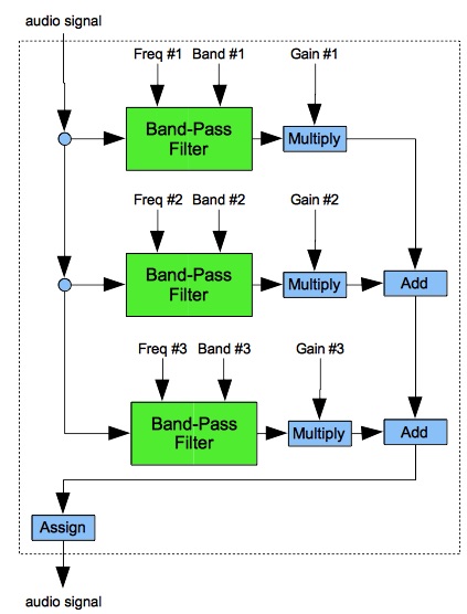
Figure 10 diagrams information flow in a Sound instrument for 3-band equalization. I realize that many older readers will regard my Equalizer components as hugely extravagant. However, the days are long past when large mainframe operations charged for computer time by the second. Neither am I greatly concerned that these components may require 8 to 12 seconds to produce sounds of merely 4 seconds duration.
To do equalization properly, each band-pass filter should have flat response through the flat frequency band and strong suppression elsewhere. However, because I was unsuccessful finding a high-pass filter that worked for me, I made do with bell-shaped response curves. The down side of making do in this way is substantial bleed over between frequency bands. This means that if you want your spectrum to change steeply between two adjacent bands, you'll need to introduce additional filtering into the stack.
The 3-band template shown in Figure 9
is expanded to 16-band equalizers in instruments from NoiseOrch.xml:
Instrument #17: Linear Equalizer and Instrument #18: Logarithmic Equalizer.
The text that follows feeds full-spectrum noise from Instrument #1: Classic Noise
through Instrument #18: Logarithmic Equalizer and through additional filters in attempts to match each of
the five noise-color spectra listed above.
Table 1 details the 16 frequency bands implemented by Instrument #18. The values in row 2 present the frequencies calculated by the instrument relative to a Nyquist limit of 22050 Hz., while those in row 3 present corresponding logarithmic values on the cents scale. Notice that between consecutive bands the frequency ratios are 1.619 to 1, which works out to 697 cents (almost, but not quite, a perfect fifth). Instrument #18 sets the width of each band is set equal to the band's frequency.
Region 1 2 3 4 5 6 7 8 9 10 11 12 13 14 15 16 Frequency 16.00 25.91 41.95 67.92 110.0 178.1 288.3 466.8 755.8 1224 1981 3208 5195 8411 13618 22050 Cents 0 695 1390 2086 2781 3476 4171 4867 5562 6257 6952 7648 8343 9038 9733 10430
Table 1: Frequency bands for Instrument #18: Logarithmic Equalizer.
As it happens, Instrument #18 is usable for finely adjusting a spectrum which already has the rough characteristics one is looking for. An example is the spectrum shown in Figure 7 (c), which is fairly flat over the audio range but a bit too strongly disposed toward the higher frequencies. It would have been great if I could have simply extracted dB levels for 16 in Figure 7 (c) (one region for each equalizer frequency band) and then converted each level into a gain. I tried that, but the equalizer greatly over-compensated.
The remainder of this heading will go about explaining how I sought workable gain multipliers using methods of trial and error. If you'd rather not wade through these details, you can skip ahead now to the specific treatment of white noise.
My trial-and-error process centered with a Java program. The program accepted among its inputs an array of 16 levels, expressed in decibels. It produced as output a note list. The note list would in turn generate a wave file, from which the Wave-File Viewer would render a Bode plot. I would eyeball this Bode plot to verify that the frequency curve had no bumps or dips. If a certain frequency band fell on a bump, I would tweak the corresponding level down, while if a band fell at a dip, I would tweak the level up. I would then request a new note list and repeat the evaluation.
The formula for converting the level li for the ith equalization band with frequency fi into the corresponding gain value gi was:
| gi | = |
|
Once I had gotten past white noise, the evaluation step took on the additional task of measuring the slope of the Bode plot in decibels per octave. This was done by selecting points along the trend line (one point on the left and one on the right) and plugging the coordinates into a formula I had set up in a spreadsheet. I also used the spreadsheet to to set up the level array in a manner allowing me to enter data in certain cells and calculate the remaining values using linear interpolation.
Noise Colors: White
White noise is the static you get from a radio tuned between channels. According to Wikipedia, the spectrum of white noise contains equal energy in each octave, which means a straight horizontal line on a Bode (log/log) plot.
My effort to produce white noise began by selecting a sample rate to 44100 Hz. (CD standard), which encompasses the full range of
audible frequencies.
The sound source (note #2) is the Noise unit with its cutoff frequency set to the
Nyquist limit of 22050 Hz.
This produces the spectrum seen previously as Figure 7 (c), which then passes through
Instrument #18: Logarithmic Equalizer (note #4) using trial-and-error gain values.
The resulting signal, written to file NoiseWhite.wav, has the spectrum plotted in Figure 11 (a).
|
||
| Listing 3 (a): Note list to produce 4 seconds of white noise. To hear a realization, click here. | Figure 11 (a): Bode plot for the white noise generated by Listing 3 (a). |
Noise Colors: Pink
According to Wikipedia, the spectrum of pink noise diminishes in proportion to frequency, which is why pink noise is also known as (1/f) noise. The drop-off rate for pink noise is -3 dB per octave.
The note list given in Listing 3 (b) again employs a 44100 Hz. sample rate. The sound source is Instrument #1: Classic Noise with a cutoff frequency of 13230 Hz. Coarse spectrum shaping is accomplished by Instrument #11: Low Pass, which has been shown elsewhere on this site to produce a drop-off rate of -2.9 dB/octave. Fine spectrum shaping is imposed by Instrument #18: Logarithmic Equalizer with gain values selected by trial-and-error. Figure 11 (b) presents a Bode plot of the resulting audio file.

|
||
| Listing 3 (b): Note list to produce 4 seconds of pink noise. To hear a realization, click here. | Figure 11 (b): Bode plot for the pink noise generated by Listing 3 (b). |
Noise Colors: Brown
According to Wikipedia, the spectrum of brown noise diminishes in proportion to the square of the frequency, giving a drop-off rate of -6 dB per octave. The resulting sound is regarded as soothing and a good masker of environmental noise. However the name “brown noise” lacks appeal. Products such as the Tranquil Moments White Noise Sound Machine for Baby very likely generate brown noise rather than white noise.
In the note list given in Listing 3 (c), the sound source is Instrument #1: Classic Noise with a cutoff frequency of 11025 Hz. Coarse spectrum shaping is accomplished by four passes through Instrument #11: Low Pass. Fine spectrum shaping is imposed by Instrument #18: Logarithmic Equalizer with gain values selected by trial-and-error. Figure 11 (c) presents a Bode plot of the resulting audio file.

|
||
| Listing 3 (c): Note list to produce 4 seconds of brown noise. To hear a realization, click here. | Figure 11 (c): Bode plot for the brown noise generated by Listing 3 (c). |
Noise Colors: Blue
I have misplaced the link to a web site where an author suggests that blue noise and violet noise are pretty much theoretical constructs since they are even less pleasant to experience than white noise. The sound of blue (azure) noise noise (linear Bode plot sloped at +3 dB/octave) can be approximated by processing Noise output through a FilterBandPass2b unit with the peak frequency set to 18000 Hz. (or half the sample rate, whichever is smaller) and the bandwidth set to 3200 Hz. This happens in Listing 4. I think the result from Listing 4 matches the Wikipedia sample pretty well.
In the note list given in Listing 3 (d), the sound source is Instrument #2: Balanced-bit Noise, which was discussed previously under the Balanced-bit Noise heading. with a cutoff frequency set to the Nyquist limit of 22050 Hz. As shown previously in Coarse spectrum shaping is accomplished by four passes through Instrument #11: Low Pass. Fine spectrum shaping is imposed by Instrument #18: Logarithmic Equalizer with gain values selected by trial-and-error. Figure 11 (c) presents a Bode plot of the resulting audio file.
|
||
| Listing 3 (d): Note list to produce 4 seconds of blue noise. To hear a realization, click here. | Figure 11 (d): Bode plot for the blue noise generated by Listing 3 (d). |
Noise Colors: Violet
The sound of violet noise noise (linear Bode plot sloped at +6 dB/octave) can be approximated by processing
Noise output through a FilterBandPass2b unit with the peak frequency
set to 18000 Hz. (or half the sample rate, whichever is smaller) and the bandwidth set to 3200 Hz.
This happens in Listing 7, the results of which may be compared to the corresponding
Wikipedia sample. Notice that the amplitude parameter
for note #1 has been scaled back from 24000 to 10000. The higher amplitude level produced many clipped samples.
I tried generating violet noise using the configuration shown in Listing 4 with bandwidths as narrow as
800 Hz. and even 200 Hz., but the results did not satisfy.

|
||
| Listing 3 (e): Note list to produce 4 seconds of violet noise. To hear a realization, click here. | Figure 11 (e): Bode plot for the violet noise generated by Listing 3 (e). |
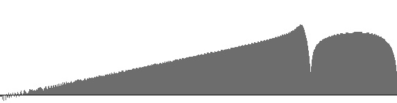
| Listing 4 (a): Band-pass noise produced by filtering (1st sound) and by sine-wave modulation (2nd sound). The center frequency is 440 Hz. and the bandwidth is 10 Hz. To hear a realization, click here. |
| Listing 4 (b): Band-pass noise produced by filtering (1st sound) and by sine-wave modulation (2nd sound). The center frequency is 440 Hz. and the bandwidth is 100 Hz. To hear a realization, click here. |
| Listing 4 (c): Band-pass noise produced by filtering (1st sound) and by sine-wave modulation (2nd sound). The center frequency is 440 Hz. and the bandwidth is 1000 Hz. To hear a realization, click here. |
Band-Pass Noise
The orthodox method for producing band-pass noise is to pass full-spectrum noise through band-pass filtering.
This can be done under NoiseOrch.xml using Instrument #1: Noise Source
and Instrument #13: Band Pass BW.
Alternatively, The Technology of Computer Music suggests generating band-pass noise by using low-band noise to amplitude-modulate a sine wave. The authors claim that this method generates noise in a band. The band's center frequency is determined by the frequency of the modulated wave, while the bandwidth is twice the noise source's cutoff frequency. We will now test that claim.
Listing 4 (a) through Listing 4 (c) generate pairs of sounds generated in the first instance using a band-pass filter and in the second instance using a modulated sine wave. In the comments, “BW” indicates Butterworth while “B/W” indicates bandwidth. The center frequencies in all three examples are 440 Hz. The bandwidths widen from 10 Hz. in Listing 4 (a) through 100 Hz. in Listing 4 (b) to 1000 Hz. in Listing 4 (c).
When I first tried this comparison I used just one note for Instrument #13: Band pass BW. As a result the first sound of each pair was very noisy around the edges. Doubling up the filter bank produced a fairly convincing match for narrow (10 Hz.) bandwidths. However as the bandwidths widen out the quality of sound diverges.
You can judge for yourself by listening to the sound examples provided for Listings 4 (a), 4 (b), and 4 (c). My own conclusion is that orthodox filtering and sine-wave modulation are not equivalent. I can't say for sure what differs between the two results, though I speculate that the filtering method — despite the double-filter cascade — still permits noise to leak through in the lower and upper stop bands. (You can test my speculation by repeating the wide-bandwidth comparisons with additional filters.) Even though the results differ, the results produced here by sine-wave modulation are definitely band-limited and definitely noisy. Thus the claim made by The Technology of Computer Music is verified, at least technically.
Vocal Fricatives
Fricative consonants are sustained noise sounds produced by the human vocal tract. This and the next heading focus on unvoiced fricatives, which result from turbulent air flow. Such turbulence can be produced either by forcing air through a constriction or by directing it around an obstacle.
A table including fricatives used in English is provided here.
Speech-synthesis systems have been around for decades, and fricative sounds were being synthesized right from the beginning.
However, my own internet search for ways of synthesizing fricative consonants yielded many unproductive hits.
For example, several sites contended that one could synthesize fricatives simply by processing brown noise
through a single formant filter, and that the frequency of the formant peak was enough to differentiate specific consonants.
I tried that, and found not one that delivered convincing sounds.
For another example, many sites provide sonograms.
However the fricative portions of these sonograms generally appear to my eyes as nothing more than a smear;
about the only thing one can see for sure is that s (as in “simple”) and ∫
(as in “should”) sounds are louder than f (as in “fox”)
and θ (as in “through”) sounds.
Pole-Zero Matching
Table 2: Frequency (Hz.) and bandwidth (also Hz.) of poles and zeros for description of the fricatives [
f, s, ş,
ç]. Checked poles and zeros enter the approximation used for synthesis.
Source: J. Mártony, “On the synthesis and perception of voiceless fricatives”,
Quarterly Progress and Status Report, Department for Speech, Music, and Hearing, KTH Royal Institute of Technology, Stockholm, Sweden, vol. 3,
no. 1 (1962), pp. 17-22, Table II-1 (page 18).
One promising hit in my internet search for information on fricative consonants was 1962 typescript by one J. Mártony: On the synthesis and perception of voiceless fricatives. The sounds I was able to produce after following Mártony's directions did not, to my ear, give convincing match to the consonants to which Mártony had ascribed them. Nonetheless, the sounds themselves have an organic quality which may prove compositionally useful.
At this writing I have been unable to locate biographical details about Mártony other than that Mártony wrote several articles about speech synthesis and collaborated with Gunnar Fant on the speech-synthesis machine called the “Orator Verbis Electris” (OVE).
At first reading, I thought Mártony's typescript an excellent piece of empirical work. He used rigorous analysis to obtain concrete numbers from spectral data, and he took things a step further by simplifying the results. At the end, he brought in independent listeners to confirm that his synthesized sounds did indeed sound like the consonants he started from. Mártony's typescript divides into two parts around the tabular summary reproduced here in Table 2.
The first part of the typescript presents graphs for each consonant, which Mártony obtained by spectral analysis. Pole-zero matching techniques were used to reduce each graph to the feature lists reproduced in Table 2. (The terms “pole” and “zero” come from mathematical filter theory: “poles” indicate peaks, while “zeros” indicate troughs.) Mártony further simplifies the description by eliminating “close-lying poles and zeros which usually have the effect of neutralizing each other and appear in the spectrum as a small dip followed by a peak.”
The second part of the typescript describes a “perceptual study”. Sound examples synthesized using Mártony's simplified spectra were played to listeners, who were in turn asked to identify which fricative consonant was being synthesized. I shall not report the outcome of this study since we will be making our own evaluation of Mártony's data.
Listing 7 (a): Note list to produce labiodental fricative sound using the features checked for fin Table 2. To hear a realization, click here.Figure 16 (a): Frequency-response curves for the filter bank used in Listing 7 (a). 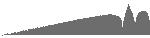
Listing 7 (b): Note list to produce alveolar fricative sound using the features checked for sin Table 2. To hear a realization, click here.Figure 16 (b): Frequency-response curves for the filter bank used in Listing 7 (b). 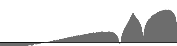
Listing 7 (c): Note list to produce prepalatal fricative sound using the features checked for ∫orşin Table 2. To hear a realization, click here.Figure 16 (c): Frequency-response curves for the filter bank used in Listing 7 (c). 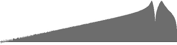
Listing 7 (d): Note list to produce palatal fricative sound using the features checked for çin Table 2. To hear a realization, click here.Figure 16 (d): Frequency-response curves for the filter bank used in Listing 7 (d).
Listing 7 (a) through Listing 7 (d) present note lists which can be used in conjunction with
NoiseOrch.xml to realize the peaks and troughs checked by Mártony's in Table 2.
In the comments, “BW” indicates Butterworth while “B/W” indicates bandwidth.
To the right of each note list is a frequency-response curve produced by using the same filters and settings as the note list.
Quite frankly, even though the peaks and troughs fall where Mártony places them, the graphs presented here look very different from the graph's presented in Mártony's Figure II-1. (Remember that Mártony's are actual spectra, while my graphs plot the frequency-responses of the filtering networks.) When I listen to the sounds generated by Listing 7 (a) through Listing 7 (d), I do not hear the consonants Mártony indicated.
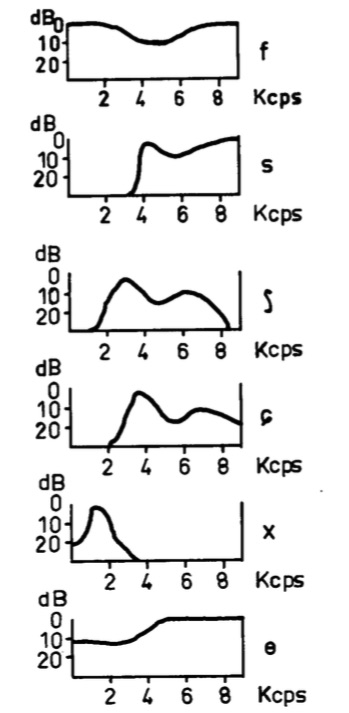
Figure 13: Schematic spectra of voiceless fricatives. Source: W. Jassem, “The formant patterns of fricative consonants”, Quarterly Progress and Status Report, Department for Speech, Music, and Hearing, KTH Royal Institute of Technology, Stockholm, Sweden, vol. 3, no. 3 (1962), pp. 6-15, Figure 1-3.
Spectrum-Matching
Another 1962 offering from the KTH Royal Institute of Technology is Wiktor Jassem's typescript, “The formant patterns of fricative consonants”. Jassem's typescript includes the spectral graphs reproduced in Figure 13. Although these hand-drawn graphs are crude compared to modern computer graphics, they digest spectral data analyzed from speakers of Swedish, English, and Polish, which the typescript reproduces in tabular formats.
The first thing to notice about Figure 13 is that Jassem's graphs plot the log of amplitude (expressed in decibels) against frequency. This is the typical way of plotting spectral graphs in the speech synthesis literature.
The second thing to notice about Figure 13 is that Jassem's graphs extend up only to 10 kHz, which is about half an octave short of the upper limit of human pitch perception. Jassem obtained his data using the RASSLAN spectrum analyzer at the Swedish Royal Institute of Technology, so we can conclude that RASSLAN operated at a 20 kHz sample rate. This was very respectable A/D conversion rate for the time, and seems to have been sufficient for Jassem's purposes. However because the spectrum-matching efforts described under this heading employ the audio CD standard rate, the graphs produced here will include an additional 12 kHz above Jassem's graphs, over which range all frequencies will be damped.
Before proceeding, it is important to stipulate that there are other ways to synthesize fricative sounds, and that some of these other approaches are far more efficient than the spectrum-fitting approach described under the present heading. In particular, Dennis H. Klatt's 1980 “Software for a cascade/parallel formant synthesizer” (J Acoust Soc Am 67, pp. 971-995) synthesizes unvoiced fricatives by processing noise through several “formant resonators in parallel” (italics mine) using frequency and gain values I have not so-far been able to obtain. Also there are methods such as linear predictive coding which can be used to deduce coefficients for an n-pole filter through analysis of a sound source. This latter approach obviates any need for a human to inspect the spectral graph.
I choose to pursue fricative speech synthesis using direct spectrum matching despite its inefficiency, which is due mostly to my use of Instrument #17: Linear Equalizer for fine spectral adjustments. I do this because working directly with noise spectra provides insight into the nature of fricative sounds. In particular it helps one to extrapolate from known fricatives to related sounds which are not spoken (at least not in English) but which nonetheless offer compositional possibilities.
First in Jassem's set of graphs is the f sound (as in
“fat”).
Jassem's spectrum for f is very broad-spectrum, but with a prominent dip
in the middle.
Listing 6 (a) details the note stack used to reproduce this spectrum for f.
The source sound is produced using Instrument #1: Classic Noise with a cutoff frequency set to the Nyquist limit.
Instrument #15: Band Reject imposes a dip around 4400 Hz. with an 1100 Hz. bandwidth.
Recall that under Taming the Notch Filter we found that notch filtering
causes an inadvertent increase in gain as frequencies rise above the notch. Listing 6 (a) mitigates this side effect by
processing the signal twice through Instrument #11: Low Pass with cutoff frequencies of 11000 Hz.
The final filtering step in Listing 6 (a) is to process the signal through
Instrument #17: Linear Equalizer for fine adjustment, with gain values selected by trial and error.
The spectrum thus produced is plotted in Figure 14 (a).

|
||
Listing 6 (a): Note list to synthesize 4 seconds of the unvoiced labiodental fricative f following Jassem's spectrum in Figure 13.
To hear a realization, click here.
|
Figure 14 (a): dB/frequency spectrum for the f noise generated by Listing 6 (a).
|
Second in Jassem's set of graphs is the s sound (as in “sip”).
Jassem's spectrum for s consists of a damped low-frequency region, a moderately wide mid-range peak, and a broad peak at the top of the
range. Such high-frequency emphasis gives the s sound its characteristic hiss.
Listing 6 (b) details the note stack used to reproduce the spectrum for s.
This particular effort cries out for a good Butterworth high-pass filter, but having no workable option Listing 6 (b) makes
do by processing the noise
sound twice through Instrument #15: Band Reject with a notch frequency of 3000 Hz. and a bandwidth set wide (1000 Hz.).
Applying the approach taken by Mártony, the mid-range peak is produced by combining
Instrument #13: Band Pass BW centered at 4200 Hz. with a narrow-band Instrument #15: Band Reject
centered at 5700 Hz.
Since notch filtering has the side effect of greatly enhancing gain as frequencies rise above the notch, there is no need for any additional
steps to enhance high-range frequencies. To suppress frequencies higher than 10 kHz., Listing 6 (b) processes
the signal twice through through Instrument #11: Low Pass.
All this is subject to fine adjustment using Instrument #17: Linear Equalizer.
The resulting spectrum is shown in Figure 14 (b), which deviates from Jassem's graph in two ways:
A bump in the low frequency region (all well below the -20dB attenuation level), and a small notch at the summit of the high-frequency
peak. Just didn't manage to adjust those features out, even after zeroing out the first five equalization bands.
|
||
Listing 6 (b): Note list to synthesize 4 seconds of the alveolar fricative s following Jassem's spectrum in Figure 13.
To hear a realization, click here.
|
Figure 14 (b): dB/frequency spectrum for the s noise generated by Listing 6 (b).
|
Third in Jassem's set of graphs is the ∫ sound (as in “sure”).
Jassem's spectrum for ∫ is of a type with his spectrum for s: a damped region followed by two peaks.
However this time first peak falls in the lower mid range, the second peak falls in the upper mid range, and a larger proportion of energy
concentrates in the lower peak.
Listing 6 (c) details the note stack used to reproduce the spectrum for ∫.
Once again there is a damped low-frequency region that begs for high-pass filtering, but which Listing 6 (b)
accommodates by using Instrument #15: Band Reject with a notch frequency of 1000 Hz.
The lower peak is obtained by cascading Instrument #13: Band Pass BW centered at 3000 Hz. into
Instrument #15: Band Reject notched at 4300 Hz. For the upper peak, the note stack employs
Instrument #14: Band Pass FLT centered at 6500 Hz. Processing the result twice through Instrument #11: Low Pass
with cutoff frequency of 6000 Hz. dampens out any high-frequency gain.
The topmost frequency for Instrument #17: Linear Equalizer
is brought down to 8000 Hz., zeroing out the first four equalization bands.
The resulting spectrum is shown in Figure 14 (c).
|
||
Listing 6 (c): Note list to synthesize 4 seconds of the prepalatal fricative ∫ following Jassem's spectrum in Figure 13.
To hear a realization, click here.
|
Figure 14 (c): dB/frequency spectrum for the ∫ noise generated by Listing 6 (c).
|
Fourth in Jassem's set of graphs is the ç sound (as in “chair”).
The spectrum for ç is an upward-shifted version of the spectrum for ∫: a damped region with one peak
short of 4000 Hz. and a second peak at around 7000 Hz.
Listing 6 (d) details the note stack used to reproduce the spectrum for ç.
The damped low-frequency region is accommodated using Instrument #15: Band Reject with a notch frequency of 2000 Hz.
The lower peak is obtained by cascading Instrument #13: Band Pass BW centered at 4000 Hz. into
Instrument #15: Band Reject notched at 5500 Hz. For the upper peak, the note stack employs
Instrument #14: Band Pass FLT centered at 7000 Hz. Processing the result twice through Instrument #11: Low Pass
with cutoff frequency 15000 Hz. dampens out any high-frequency gain.
Fine processing by Instrument #17: Linear Equalizer
employs a maximum frequency of 8000 Hz., zeroing out the first six equalization bands.
The resulting spectrum is shown in Figure 14 (d).

|
||
Listing 6 (d): Note list to synthesize 4 seconds of the palatal fricative ç following Jassem's spectrum in Figure 13.
To hear a realization, click here.
|
Figure 14 (d): dB/frequency spectrum for the ç noise generated by Listing 6 (d).
|
Fifth in Jassem's set of graphs is the x sound (as in the Scottish “loch”).
The spectrum for x is of its own type, with a narrow low-frequency trough followed by just one narrow low-frequency band peaking below 2000 Hz.
Listing 6 (e) details the note stack used to reproduce the spectrum for x.
The initial low-frequency trough is accommodated using Instrument #15: Band Reject with a notch frequency of 200 Hz.
and very narrow bandwidth.
The lower peak is obtained using Instrument #13: Band Pass BW centered at 1500 Hz.
Processing the result twice through Instrument #11: Low Pass
with cutoff frequency 3000 Hz. dampens out all high-frequency content.
The fine-adjustment pass through Instrument #17: Linear Equalizer complements the low-pass steps
steps by bringing its topmost frequency band the way down to 3000 Hz. Instrument #17 complements
the low-frequency notch by zeroing out the first five equalization bands.
The resulting spectrum is shown in Figure 14 (e).
|
||
Listing 6 (a): Note list to synthesize 4 seconds of the velar fricative x following Jassem's spectrum in Figure 13.
To hear a realization, click here.
|
Figure 14 (a): dB/frequency spectrum for the x noise generated by Listing 6 (d).
|
Sixth and bottommost in Jassem's set of graphs is the θ sound (as in “thin”).
The spectrum for θ bears a familial resemblance to the spectrum for f in that spectral energy is diffused over
the entire range from 0 to 10 kHz. The spectrum for θ also contains a broad dip; however in this case the dip is located
in the low-frequency region.
Listing 6 (f) details the note stack used to reproduce the spectrum for θ.
The initial low-frequency dip is accommodated using Instrument #15: Band Reject with a notch frequency of 3000 Hz.
and wide bandwidth.
Processing the result twice through Instrument #11: Low Pass
with cutoff frequency 11000 Hz. dampens out high frequency content.
The fine-adjustment pass through Instrument #17: Linear Equalizer spans the full range from 0 to 10 kHz. with
gain values chosen by trial and error to obtain a flat log(amplitude)/frequency response between 5 and 10 kHz.
The resulting spectrum is shown in Figure 14 (f).

|
||
Listing 6 (e): Note list to synthesize 4 seconds of the dental fricative θ following Jassem's spectrum in Figure 13.
To hear a realization, click here.
|
Figure 14 (e): dB/frequency spectrum for the θ noise generated by Listing 6 (e).
|
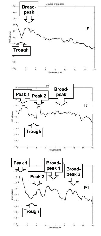
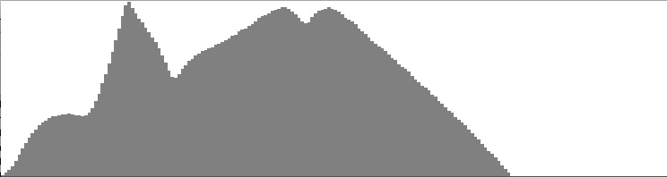
Figure 15: Plosive Spectra. Source: Marisa Lobo Lousada, Luis M. T. Jesus, and Daniel Pape, Estimation of stops' spectral place cues using multitaper techniques (DELTA: Documentação de Estudos em Lingüística Teórica e Aplicada, vol. 28, no. 1, 2012, pp. 1-26), Figure 4.
Plosive Bursts
Plosive consonants are among the most complex sounds produced by the human voice. Each single plosive phoneme combines an articulatory silence, a percussive noise burst, and an aspiration (for unvoiced plosives), with rapid formant transitions. The present heading is devoted specifically the noise spectrum of the percussive burst. It will be left to a more advanced page, “Speech Synthesis: Plosives” to bring everything together.
English produces plosive bursts at three locations along the vocal tract: labial represented by p,
dental represented by t, and guttural represented by k and g.
These three consonants are known as the unvoiced plosives. Just by uttering them one can deduce that the spectral energy
for p concentrates more in the lower frequency range, the energy for t is upper range,
and the energy for k is mid-range. Some early sources in fact suggest synthesizing plosive bursts using the methods
described above for band-pass noise; however, I do not find this approach remotely convincing.
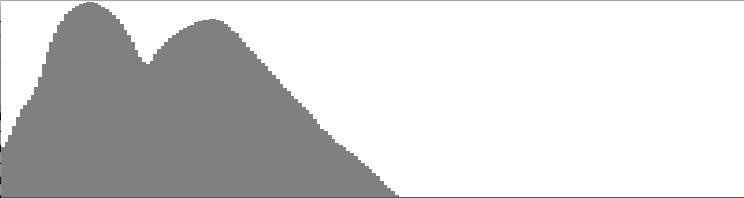
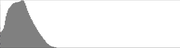
Figure 15 reproduces spectral graphs presented in 2012 by Lousada, Jesus, and Pape (LJP) for p,
t, and k. The goal of the present heading is to replicate the broad features of these three spectra.
-
The LJP spectrum for
pis initiated by a peak at 0 Hz., a trough at around 1000 Hz. and a peak at around 2000 Hz. the second peak initiates a gradual roll-off of -2.4 dB per 1000 Hz. to the topmost graph frequency of 16 kHz. Listing 7 (a) details the combination of band-pass, notch (band-reject) and low-pass filters used to obtain these features, with results shown in Figure 16 (a). -
The LJP spectrum for
tis also initiated by peak-trough-peak pattern, but with frequencies in this case shifted upward to 1750 Hz. (peak1), 3000 Hz. (trough) and 4500 Hz. (peak2). Following this is a plateau, about 15 dB down from peak levels and extending upwards to around 13 kHz. Listing 7 (b) details the combination of band-pass, notch (band-reject) and low-pass filters used to obtain these features, with results shown in Figure 16 (b) -
The LJP spectrum for
kalso begins peak-trough-peak, with the trough in roughly the same location astand a wider peak-to-peak spacing: 500 Hz. (peak1), 3000 Hz. (trough), 4500 Hz. (peak2). Following this the region from 6 to 13 kHz could be characterized either as two broad peaks or an interrupted plateau with a trough at 9500 Hz. Listing 7 (c) details the combination of band-pass, notch (band-reject) and low-pass filters used to obtain these features, with results shown in Figure 16 (c)

Listing 7 (a): Note list to mimic the rough features of the spectrum shown for pin Figure 15. To hear a sustained realization, click here. To hear a burst, click here. To hear the burst with aspirated vowels, click here.Figure 16 (a): dB/frequency spectrum for the pburst noise generated by Listing 7 (a).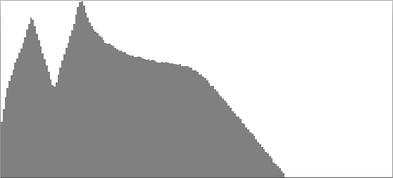
Listing 7 (b): Note list to mimic the rough features of the spectrum shown for tin Figure 15. To hear a realization, click here. To hear a burst, click here. To hear the burst with aspirated vowels, click here.Figure 16 (b): dB/frequency spectrum for the tburst noise generated by Listing 7 (b).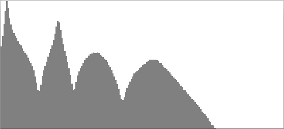
Listing 7 (c): Note list to mimic the rough features of the spectrum shown for kin Figure 15. To hear a realization, click here. To hear a burst, click here. To hear the burst with aspirated vowels, click here.Figure 16 (c): dB/frequency spectrum for the kburst noise generated by Listing 7 (c).
If you're not convinced by the plosive bursts just presented, well neither am I. It seems that the noise burst is but one low-ampltitude component of a plosive consonant. For unvoiced plosives, the other component is an aspiration which undergoes a rapid formant transition and that the nature of this transition varies according to which vowel is being approached. More about this on the page devoted to Speech Synthesis: Plosive Consonants.
Comments
-
If you have access to the Sound desktop application, then either you can view details about
NoiseOrch.xmlor you can run the examples yourself. Follow the instructions given in here to downloadNoiseOrch.xmlinto your working directory. Fire up the application. To view orchestra details, right click on the Orchestras collection, select “Open Orchestra” from the popup menu, and selectNoiseOrch.xmlin the file chooser. To realize a note list, right click on the Note Lists collection, and select “New Note List” from the popup menu. This will create an empty note list. Copy the note list from this page and paste the text into the note-list editor.
Next topic: Tone Clusters
| © Charles Ames | Page created: 2014-02-20 | Last updated: 2017-08-15 |