Operation of the Digital Oscillator

Introduction

This page explains how Oscillator units generate tones. There are several ways of implementing digital oscillators, including truncating, rounding, and interpolating. The Sound engine implements interpolating oscillator solely, but for purposes of understanding it is better first to describe the truncating implementation, then to explain the refinements introduced by the interpolating implementation. Thus the following explanation is by no means specific to the Sound engine.

Stored Waveform

All digital oscillators rely upon a stored waveform, and the explanation which follows will refer to this entity using the variable name Waveform. Waveform indiates an array of floating-point numbers, where the kth array element will be indicated as Waveform(k). Since oscillators can share waveforms, you can assume that the waveform has been passed by reference from the sound-synthesis engine into the oscillator.

For example, Figure 1 illustrates how one period of a sine wave can be represented using an array of 16 samples. Notice how the numbering begins with sample #0; a number used to indicate a particular element in an array is called an array index. Indices must always be integers. Notice also that Figure 1 includes a sample #16, that sample #16 has the same value as sample #0, and that sample #16 is not counted in the waveform length. For the moment, please regard this redundant sample as a way of indicating graphically how the waveform cycles back upon itself.

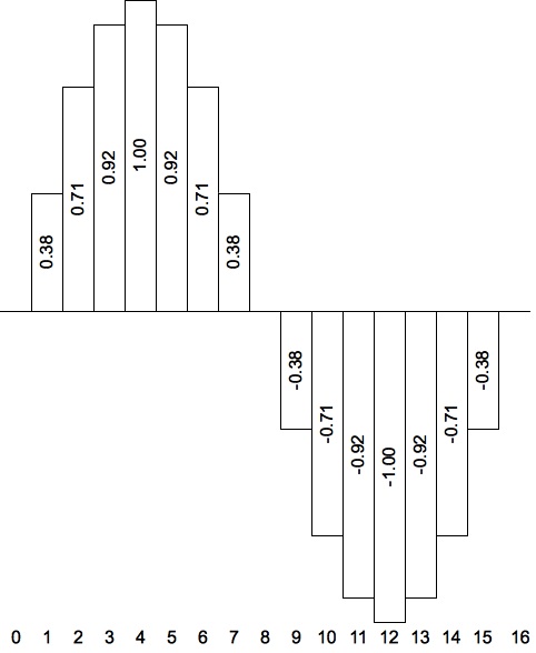
Figure 1: A sixteen-sample representation of a sine wave.

Suppose we have a sampling rate of 10,000 and wish to generate a tone with a frequency of 440 Hz. Then the oscillator will need to iterate the contents of the Waveform array 440 times over the course of 10,000 samples. This comes out to 10,000/440 = 22.727 samples per iteration. The word sampling indicates the process of selecting which stored value should be the next signal value. The immediate challenge is that we wish to select stored values from the waveform at 22-and-some equally spaced positions.

The Phase Variable

The heart of any digital oscillator is a running variable, here-named Phase, which corresponds to the phase property of a waveform. The Phase variable indicates which stored value the oscillator should use next. Since the spacing between Phase values is fractional, the variable needs to be of the floating-point type. Since we want sampling the begin with the leftmost sample in Figure 1, the initial value for Phase should be zero.

To produce a frequency of 440 Hz., the Phase variable must advance by a sampling increment calculated as follows:

(sampling increment)	=	(frequency) × (waveform length) (sampling rate)	=	440 × 16 10,000	= 0.704

The sampling increment is the factor which stretches out a stored-waveform length of 16 samples into an oscillating signal with a 22.727-sample period (16/22.727 = 0.704). The sequence of values generated by repeatedly adding a sampling increment of 0.704 to Phase is detailed is the second column of Table 1.

It is clear from Figure 1 that the sample value should be 0.00 when the Phase is 0 and that the sample value should be 0.38 when the Phase is 1. However, what should the sample value be when the Phase is 0.704? This question will be answered in one quick-and-dirty way by the truncating oscillator and in a second, slower-and-cleaner way by the interpolating oscillator.

Table 1 details the calculations a digital oscillator would make using the waveform shown in Figure 1 with a sampling increment of 0.704. This table serves double duty for explaining the truncating oscillator and the interpolating oscillator, so for the moment please ignore the three rightmost columns.

Sample	Phase	Index	Waveform(Index)	Waveform(Index+1)	Residue	Interpolation
0	0.00	0	0.00	0.38	0.00	0.00
1	0.70	0	0.00	0.38	0.70	0.27
2	1.41	1	0.38	0.71	0.41	0.51
3	2.11	2	0.71	0.92	0.11	0.73
4	2.82	2	0.71	0.92	0.82	0.88
5	3.52	3	0.92	1.00	0.52	0.96
6	4.22	4	1.00	0.92	0.22	0.98
7	4.93	4	1.00	0.92	0.93	0.93
8	5.63	5	0.92	0.71	0.63	0.79
9	6.34	6	0.71	0.38	0.34	0.60
10	7.04	7	0.38	0.00	0.04	0.36
11	7.74	7	0.38	0.00	0.74	0.10
12	8.45	8	0.00	-0.38	0.45	-0.17
13	9.15	9	-0.38	-0.71	0.15	-0.43
14	9.86	9	-0.38	-0.71	0.86	-0.66
15	10.56	10	-0.71	-0.92	0.56	-0.83
16	11.26	11	-0.92	-1.00	0.26	-0.94
17	11.97	11	-0.92	-1.00	0.97	-1.00
18	12.67	12	-1.00	-0.92	0.67	-0.94
19	13.38	13	-0.92	-0.71	0.38	-0.83
20	14.08	14	-0.71	-0.38	0.08	-0.68
21	14.78	14	-0.71	-0.38	0.78	-0.45
22	15.49	15	-0.38	0.00	0.49	-0.19
23	0.19	0	0.00	0.38	0.19	0.07
24	0.90	0	0.00	0.38	0.90	0.34
25	1.60	1	0.38	0.71	0.60	0.58
26	2.30	2	0.71	0.92	0.30	0.77
27	3.01	3	0.92	1.00	0.01	0.92
28	3.71	3	0.92	1.00	0.71	0.98
29	4.42	4	1.00	0.92	0.42	0.97
30	5.12	5	0.92	0.71	0.12	0.89
31	5.82	5	0.92	0.71	0.82	0.75
32	6.53	6	0.71	0.38	0.53	0.54
33	7.23	7	0.38	0.00	0.23	0.29
34	7.94	7	0.38	0.00	0.94	0.02
35	8.64	8	0.00	-0.38	0.64	-0.24
36	9.34	9	-0.38	-0.71	0.34	-0.49
37	10.05	10	-0.71	-0.92	0.05	-0.72
38	10.75	10	-0.71	-0.92	0.75	-0.87
39	11.46	11	-0.92	-1.00	0.46	-0.96
40	12.16	12	-1.00	-0.92	0.16	-0.99
41	12.86	12	-1.00	-0.92	0.86	-0.92
42	13.57	13	-0.92	-0.71	0.57	-0.80
43	14.27	14	-0.71	-0.38	0.27	-0.62
44	14.98	14	-0.71	-0.38	0.98	-0.39
45	15.68	15	-0.38	0.00	0.68	-0.12
46	0.38	0	0.00	0.38	0.38	0.15

Table 1: Digital oscillator calculations using the waveform shown in Figure 1 with a sampling increment of 0.704.

Truncating Oscillator

The quick-and-dirty solution is to allocate a new integer variable called Index, to populate Index by lopping off (truncating) the fractional part of Phase, and then use Index to identify a stored value in the Waveform array. The sequence of values obtained by deriving Index from Phase in this manner is detailed is the third column of Table 1.

Notice in Table 1 that the Phase value for sample #22 is 15.49, or more accurately, 15.488 . Now 15.488 + 0.704 - 16 = 16.192, the integer part of which is 16. However the valid indices for the Waveform array run from 0 to 15. We must now consider what should be done when the running Phase reaches or surpasses the waveform length of 16 samples.

A brute-force solution would be to reset the Phase value to zero. This would have the effect of reducing the period of oscillation from 22.727 samples to 22.000 samples — with a corresponding frequency of 455 Hz.! The brute-force solution is therefore not viable.

Since we cannot discard the fractional residue of 0.192, we must instead carry it forward into the Phase value for sample #23. Carrying residues forward in this manner means that number of samples required to complete a full oscillation will be:

• 23 in the first cycle, leaving a residue of 0.192,
• 23 in the second cycle, leaving a residue of 0.384, and
• 23 in the third cycle, leaving a residue of 0.576.
• 22 samples in the fourth cycle, since the accumulated residue 0.576+0.192 = 0.768 exceeds a full sample's worth of residue, which is 0.704.

By inserting a 22-sample oscillation between every 2.66 23-sample oscillations, the average number of samples per oscillation comes out to (2.66×23 + 1×22)/(2.66 + 1) = 22.727, which is the period of oscillation required for a 440 Hz. tone.

Columns 1 through 4 of Table 1 are described below:

• The leftmost column identifies which sample number the remaining columns pertain to.
• The Phase column starts at zero. Each successive entry increments the previous entry by 0.704. Whenever the Phase threatens to fall outside the range from 0.00 (inclusive) to 16.00 (exclusive), the oscillator wraps it back into range. This happens for sample #23 and sample #46.
• The numbers in the Index column are obtained by truncating the Phase value to the next lower integer.
• The numbers in the Waveform(Index) column, are obtained by using the Index variable to look up values in the Waveform array. The sequence of values in the Waveform(Index) column are presented graphically in Figure 2.

Figure 2 shows the oscillator signal generated using the truncating method. The shape is especially blocky (adding noise to the signal) because the waveform length is so short. My Sound engine does not actually offer a truncating option, but it is very instructional to see how the waveform spreads out when the sampling increment is less than unity.

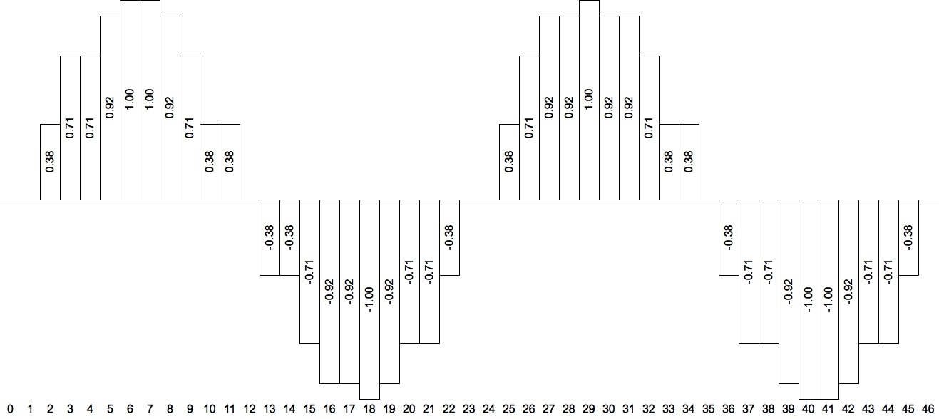
Figure 2: Graphic display of truncating oscillator output using the Waveform(Index) column from Table 1.

Video 1-1 and Video 1-2 animate the waveform lookups performed by a truncating digital oscillator. Each animation cascades two stages. The left-side stage labeled Oscillator looks up samples from a stored waveform. The vertical scale gives the instantaneous signal value, while the horizontal scale of the waveform is 10 pixels per sample. The right-side stage labeled Output is a signal queue. It carries through the Oscillator's vertical scale, but reduces the horizontal scale to one pixel per sample.h Each frame of the animation scrolls the Output contents rightwards by one pixel, allowing the newly generated sample to be plotted in the leftmost position. The samples thus plotted proceed from newer samples on the left to older samples on the right, reversing theorder of presentation normally expected a time-series graph.

800 samples are generated over the course of each video. Since the Output queue only has room for 640 samples, the earliest 160 samples have fallen off the right side of the queue when the video is done.

The operation of the Oscillator stage is indicated by the arrow which first extends vertically from the the x-axis to the waveform value and which continues horizontally over to the Output queue. The starting point of this arrow indicates the current Phase value, which wraps around from 0 (inclusive) on the left to 16 (exclusive) on the right.

The sampling increment for Video 1-1 is 0.0618, which means that the vertical portion of the Oscillator-to-Output arrow advances rightward at a rate of 0.0618×10=0.618 pixels per frame. The number of frames required to complete one oscillation is 16/0.0618=258.9, which means that Phase will cycle from 0 to 16 800/258.9=3.1 times over the duration of the video. The Phase will linger over each Index for 1/0.0618=16.2 samples, so the Output wave proceeds as a series of horizontal steps, each 16 (sometimes 17) samples wide.

Video 1-1: Truncating sine-tone generation with a sampling rate of 0.618 pixels per frame.

The sampling increment for Video 1-2 is 0.272, which means that the vertical portion of the Oscillator-to-Output arrow advances rightward at a rate of 0.272×10=2.72 pixels per frame. The number of frames required to complete one oscillation is 16/0.272=58.8, which means that Phase will cycle from 0 to 16 800/58.8=13.6 times over the duration of the video. The Phase will linger over each Index for 1/0.272=3.7 samples, so the Output wave proceeds as a series of horizontal steps, each 4 (sometimes 3) samples wide.

Video 1-2: Truncating sine-tone generation with a sampling rate of 2.718 pixels per frame.

Interpolating Oscillator

The signals produced by truncating digital oscillators in Figure 2, in Video 1-1, and in Video 1-2 have been characterized by plateaus, interrupted by fairly dramatic sample-to-sample transitions, and the result of this discontinuity is quantization noise. The most direct way to reduce quantization noise is to increase the length of the Waveform array; this action has the added advantage of coping with higher harmonics: a 16-sample waveform can accomodate only up to harmonic #8, while a 512-sample waveform can accomodate up to harmonic #256.

Another way to reduce quantization noise is to smooth out the transitions between stored-sample values. Instead of holding on to one stored value until the Index variable advances to a new array element, the oscillator can look ahead to the next stored sample and plot values along a line from one stored-sample value to the next. The process of estimating unknown values by plotting lines between known values is called linear interpolation.

All the features of the truncating oscillator carry through into the interpolating oscillator: the Waveform array, the Phase variable for selecting stored-sample values, and Index variable used to convert Phase into an array index, and the current stored-sample value Waveform(Index). Interpolation requires additionally that the oscillator know the next stored-sample value Waveform(Index+1), and to know how far along it is between the current stored value and the next. For for this purpose the interpolating oscillator introduces a floating-point variable named Residue. This variable holds the fractional part of Phase; that is,

Residue = Phase - Index.

The sequence of next-stored-samples residues appear in columns 5 and 6, respectively, of Table 1. The interpolated sample value in column 7 (rightmost) is calculated using the formula:

Interpolation = Waveform(Index) + Residue×(Waveform(Index+1) - Waveform(Index))

To make this formula work requires that Waveform(Index+1) be meaningful when Index+1 equals the number of stored samples. That means appending an additional sample onto the array, where the value of the appended sample equals the value of the starting (leftmost) sample. The interpolating method for tone generation produces better signal quality than the truncating for waveforms of equal length. Interpolation happens at a cost of extra processing cycles, but in today's world of hardware floating-point accelerators that cost matters nowhere near as much as it used to.

Figure 3 shows the oscillator signal generated using the interpolating method.

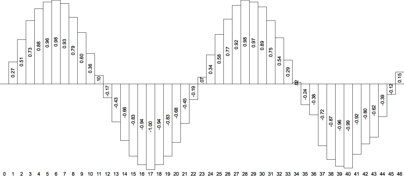
Figure 3: Graphic display of interpolating oscillator output using the Interpolation column from Table 1.

The right-side stage labeled Output is a signal queue. It carries through the Oscillator's vertical scale of intensity, but reduces the horizontal scale of time to one pixel per sample.

Video 2-1 and Video 2-2 animate the waveform lookups performed by an interpolating digital oscillator. Each animation cascades two stages. The left-side stage labeled Oscillator is much like the Oscillator in Video 1-1. The vertical scale gives the instantaneous signal magnitude, while the horizontal scale of the waveform is 10 pixels per stored value. What's new here is the thin black segmented curve which interpolates between consecutive stored-sample values. The segmented curve resembles a continuous sine graph, but if you look closely — especially in the places where the waveform changes direction — you can see that its pieced together from line segments, one for each stored sample.

The right-side stage labeled Output acts just like the Output queue Video 1-1.

800 samples are generated over the course of each video. Since the Output queue only has room for 640 samples, the earliest 160 samples have fallen off the right side of the queue when the video is done.

The operation of the Oscillator stage is indicated by the arrow which first extends vertically from the the x-axis and which continues horizontally over to the Output queue. The starting point of this arrow again indicates the current Phase value, which wraps around from 0 (inclusive) on the left to 16 (exclusive) on the right. In the present videos, however, the vertical portion of the arrow extends not to the stored value, but rather to the segmented curve.

The sampling increment for Video 2-1 is 0.0618, which means that the number of frames required to complete one oscillation is 258.9. The Phase variable will cycle from 0 to 16 3.1 times over the duration of the video. Phase will linger over each Index for 16.2 samples, so the Output wave proceeds as a series of line segments, each 16 (sometimes 17) samples wide. The resolution of the video makes this pretty much indistinguishable from a continuous sine wave.

Video 2-1: Interpolating sine-tone generation with a sampling rate of 0.618 pixels per frame.

The sampling increment for Video 2-2 is 0.272, which means that the number of frames required to complete one oscillation is 58.8. The Phase variable will cycle from 0 to 16 13.6 times over the duration of the video. Phase will linger over each Index for 3.7 samples, so the Output wave proceeds as a series of line segments, each 4 (sometimes 3) samples wide.

Video 2-2: Interpolating sine-tone generation with a sampling rate of 2.718 pixels per frame.

Foldover

Foldover also has an effect on the number of frequencies one can shoehorn into a digitized waveform. Recall that Figure 3 attains a fairly convincing representation of a sine wave storing only sixteen points. Recall also that interpolating between stored sample values greatly reduces quantization noise. However, the fact that two samples are required for each cycle of a wave means that a 16-sample stored waveform can only represent harmonics up to number 8 — and interpolation cannot remedy that situtation.

Now consider a stored waveform which incorporates harmonics beyond the fundamental. For example, consider a square wave incorporating the fundamental with relative amplitude 1, the third harmonic with amplitude 1/3, the fifth harmonic with amplitude 1/5, and the seventh harmonic with amplitude 1/7. How high can you go with this waveform?

The bad news is that each harmonic butts up independently against the Nyquist limit. So attempting to generate a square wave with a frequency of 1175 Hz. (D in the 6th octave), will need to accomodate 3525 Hz. for harmonic #3, 5875 Hz. for harmonic #5 and 8225 Hz for harmonic #7. A sampling rate is 10,000 samples per second yields a Nyquist limit of 10,000/2 = 5000 Hz., which is good for the fundamental and for harmonic #3, but not good for harmonic #5 (875 above Nyquist, yielding an alias of 4125 Hz.) or harmonic #7 (3225 above Nyquist, yielding an alias of 1775 Hz.) — not the result intended!

Video 4 animates an attempt to run a square-wave generator at frequencies higher than than the Nyquist limit. The video displays five systems running in parallel, where each system uses an oscillator to generates samples, then plots the resulting samples upon a scrolling intensity-versus-time graph. The topmost oscillator, labeled Compound Waveform, samples a complex waveform made up of harmonics #1, #3, #5, and #7. The remaining oscillators sample each of these harmonics individually.

The video again lasts 100 seconds overall. The sampling increment begins at 1/32 of the sample rate. Over the first 50 seconds it widens by equal ratios. to 1/4 of the sampling rate, then over the remaining 50 seconds the sampling increment narrows toward an ending rate of 1/32. Notice that at no time during this demonstration does the sampling increment ever exceed the Nyquist limit. The audio track which accompanies Video 3 was generated at a rate of 10,000 samples per second using an instrument similar to the one shown in Figure 2-2. The oscillator frequency again followed a contour with two exponential segments. In this case the starting and ending frequencies were 312.5 Hz. (1/32) of the sample rate, while the mid-point frequency was 2500 Hz. (1/4 of the sample rate).

The frame rate for Video 3 has been deliberately ratcheted down to 2.5 frames per second so that you can witness how the direction of angular displacement shifts from counter-clockwise to clockwise during the upward Nyquist transition (41 seconds in). At this point the audio tone stops rising and begins falling. The tone continues falling to the mid-point (50 seconds in). Here the angular displacement shifts from clockwise to counter-clockwise nominal mid-point frequency peak, occuring under foldover conditions, actually comes off as a trough. During the downward Nyquist transition (60 seconds in), the angular displacement shifts from clockwise to counter-clockwise, and the audio tone assumes its expected downard trend.

Video 4: Square-wave generation by waveform lookup. Displacements increase from N/16 initially to N/3 mid-way through, then decrease back to N/16 at the end. The legend FOLDOVER appears during frames when the sampling increment exceeds the Nyquist limit. Sample values generated during such frames appear with yellow backgrounds in the signal graph.