Fundamentals of Instrument Design
Introduction
This page explains the workings of MUSIC-N-style sound-synthesis
instruments at an elementary level.
The explanations on this page use animation to demonstrate visually how various signal-processing units work, and also describes how instruments are linked together from units. Central to all this is the digital signal, which is a stream of numerical values called samples. Audio signals such as tones and noises are distinguished from control signals such as amplitudes.
The designs presented below have their description supplemented by animations charting signal flows between units and giving visualization to the processing operations. You are assumed to be familiar with the workings of the digital oscillator and of the digital noise generator.
Signals
A digital signal quantifies ongoing fluctuations of a source using a sequence of
numerical values called samples. Each sample represents the state
of the source as of a particular moment of time. For signals processed using the MUSIC-N
family of software programs; the time interval between samples is subject to a fixed
sampling rate; however, this limit is by no means
universal.1
The designs presented below have their description supplemented by animations charting signal flows between units and giving visualization to the processing operations. Within these animations, the flow proceeds at a rate of one pixel per frame.
Audio-Rate Signals
Within the digital world, an audio signal represents sound using a sequence such as the one graphed Figure 1. This graph plots sample values along the vertical scale against time along the horizontal scale. We'll get to the color-coding of sample intensities in a bit.
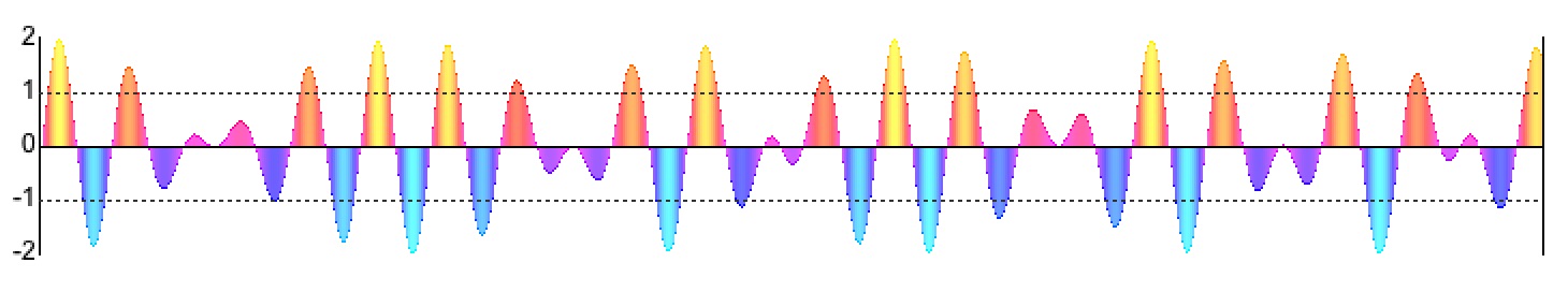
Figure 1: Audio-Rate Signal.
The transmission path for an audio signal begins digitally with a stream of numeric samples. Samples pass along at a clocked rate to a digital-to-analog converter, which transforms them into rapidly fluctuating voltages. Changing voltages create mechanical vibrations in a loudspeaker. Vibrations propagate through the air until they come up against the ear drum. Thus does a digital sample come to indicate a momentary level of air pressure, exerted upon an auditory membrane. A sample value of zero indicates the ear drum is at equilibrium, the inner pressure equalling the outer pressure. A positive sample value indicates greater external pressure while a negative sample indicates greater internal pressure. So long as these pressure differences keep to small fractions of a standard atmosphere, their exact magnitudes matter less than the way they change.
The horizontal unit of time for a digitized audio signal is determined by a sampling rate which is a fixed property of the signal as a whole. The CD standard sampling rate is 44,100 samples per channel per second. At this rate the 700 samples graphed in Figure 1 would run in around 1/63 of a second.
Physicists and mathematicians since Daniel Bernoulli have understood that every sound can be broken down into simple components called sine tones. Built into the ear is a sensor, the cochlea, which responds to different sine-tone frequencies at different locations. Nerves hooked in to each of these locations enable the cochlea to act as a frequency spectrum analyzer over the human range from 20 Hz. to some 20,000 Hz.
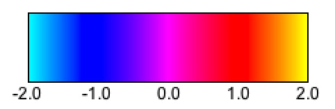
Notice that signal intensities in Figure 1 are color-coded according to the gamut shown in Figure 2, where
- Cyan indicates -2,
- Blue indicates -1,
- Violet indicates 0,
- Red indicates +1,
- Yellow indicates +2.
This color coding will be retained throughout this page, and will serve to indicate signal intensities in conditions where it would be difficult to express them graphically.
Synthesis Malfunctions
There are two things to watch for when generating audio signals. One is foldover, the other is sample overflow. My discussion of foldover had these takeaways:
To generate a tone of any frequency requires at least two samples per waveform period, one for the up phase and one for the down phase. To generate a one-second tone with a frequency of 20,000 Hz. therefore requires a sample rate of at least 40,000 samples per second. The rate for audio CD's is actually 44,100 samples per second, which builds in an extra margin of quality.
It's not only fundamental frequencies that need to be kept under the 22,100 Hz. ceiling. You have to take harmonics into account as well. The highest note on most pianos is C8, with a fundamental frequency of 4186 Hz., a second harmonic of 8371 Hz., a third harmonic of 12,558 Hz., a fourth harmonic of 16,744 Hz., a fifth harmonic of 20930 Hz., and a sixth harmonic of 25,116 Hz. The fundamental is okay, as are harmonics 2-5; however harmonic #6 exceeds the Nyquist limit of 22,100 Hz. Trying to generate that frequency will produce a fairly awful consequence.
- Trying to generate a frequency higher than the Nyquist limit produces foldover.
- Not making waveform lengths large enough to accomodate high harmonics produces foldover.
- Trying to generate a complex tone whose harmonics would overreach the Nyquist limit produces foldover.
Sample overflow results when you try generate a sample value more positive than 32764 or more negative than -32764. The signal processing units can handle such values but the engine chokes when attempting to save the sample to a audio file with a sample-size of 16 bits.
Control-Rate Signals
Control signals are signals which act to modulate the behavior of oscillators, noise generators, filters, and other audio units. For the most part, control signals change too slowly to be perceived as sound. Where audio signals tend to alternate rapidly positive and negative samples, control signals tend to remain in the non-negative range (zero indicating no sound). Control signals often unfold as a series of ramps, where one ramp's the ending sample value carries over to become the next ramp's starting value. The ramp style of control signal is what one would use to obtain effects such as crescendo, diminuendo, and glissando. Alternatively, control signals can behave as a low-frequency oscillator to obtain effects such as “vibrato, tremolo, and phasing”.
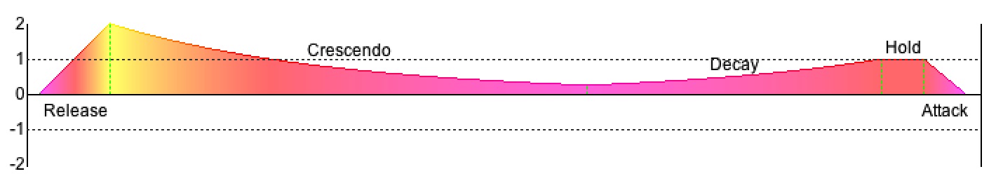
Figure 3: Control-Rate Signal.
The most common example of a control signal is an envelope generator. For example, the flavor of envelope illustrated in Figure 3 unfolds over five phases, each implemented as a ramp:
- The Attack phase rises linearly from zero at the note starting time to unit amplitude over a specified attack duration.
- The Hold phase sustains unit amplitude over a specified hold duration.
- The Decay phase drops off by equal ratios over equal units of time. This phase lasts through the note duration minus the attack duration, hold duration, and release duration.
- The Crescendo phase swells up by equal ratios over equal units of time. This phase lasts through the note duration minus the attack duration, hold duration, and release duration.
- The Release phase begins just prior to the note ending time and decends linearly from whatever amplitude happens to be in effect to zero at the note ending time. A specified release duration controls the time of descent.
The two different kinds of signal, audio and control, suggest basic principles of instrument design. The most elementary is that each signal which is generated must also be consumed, the ultimate consumer being either Output or Stereo. The next principle is that control signals come first, and are consumed in the production or modulation of audio signals.
Unit types are distinguished between signal generators and signal modifiers. The formal difference between these categories is that none of the inputs to a generator needs be a signal (and inputs which do happen to be signals are typically control signals), while at least one of the inputs to a modifier must be a signal.
Signal Arithmetic
Signal modifiers start with one or more signal inputs and transform these inputs to produce an output. When there's just one input the transformation can be presented visually as a two-dimensional graph. Within this graph,
- The input serves as the independent variable, or abscissa. This value is typically represented using the variable x.
- The output serves as the dependent variable, or ordinate. This value is typically represented using the variable y.
|
|
|
|
Figure 4-1: Identity transformation y = x.
Orientation: input-top/output-right. |
Figure 4-2: Power-of-two transformation y = 2x.
Orientation: input-left/output-bottom. |
For examples, consider the identity transformation y = x. As illustrated in Figure 4-1, the identity transformation renders as a straight line through the origin with a slope of 45°. Consider also the power-of-two transformation y = 2x. As illustrated in Figure 4-2, the power-of-two transformation renders as a curve increasing to infinity as x goes positive and diminishing to zero as x goes negative.
The y-axis will always be perpendicular to the x-axis, but we do not stipulate which axis is horizontal and which is vertical.
When there's more than one input, the transformation can still be graphed in two dimensions provided that one input is treated as primary and the remaining inputs are treated as parameters. Once specific values have been chosen for each parameter, the transformation can then be rendered using the primary input as the independent variable and the output as the dependent variable. Whenever a parameter changes, the graph must be redrawn.
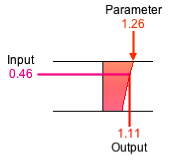
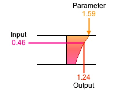
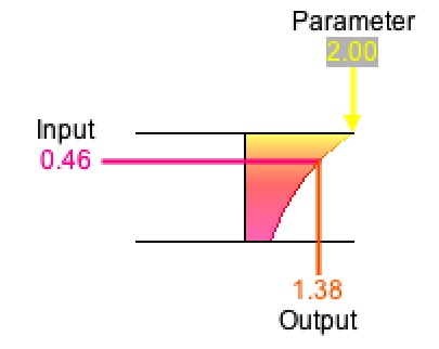
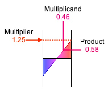
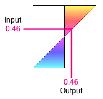
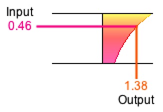
Figure 6: Multiplication y = m × x
rendered with x = 0.46 and m = 1.25.
Orientation: input-top/output-right.
Multiplication (Amplification)
Consider multiplication. Multiplication produces an output from two inputs. The primary input is called the multiplicand, the secondary input is called the multiplier, and the output is called the product. If x represents the multiplicand, m represents the multiplier, and y represents the product, then the transformation can be rendered by graphing y = m × x, which is a straight line through the origin with a slope determined by m.
The Multiply unit implements the operation
Output(K) = Input1(K) × Input2(K),
where
-
Output(K), the product, is theKth sample of the output signal, -
Input1(K), the multiplicand, is theKth sample of the primary input signal, and -
Input2(K), the multiplier, is theKth sample of the secondary input signal.
|
|
|
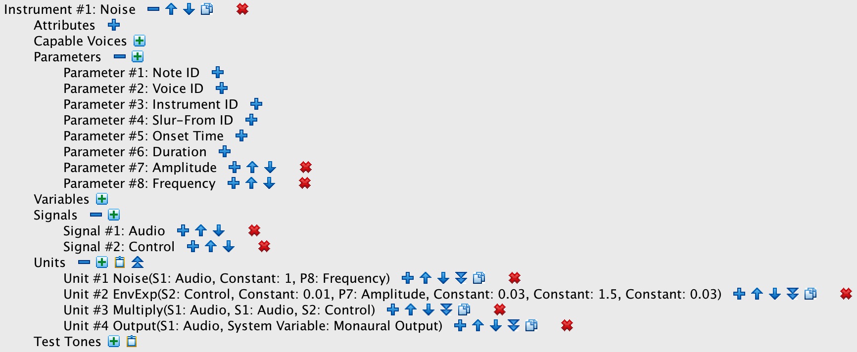
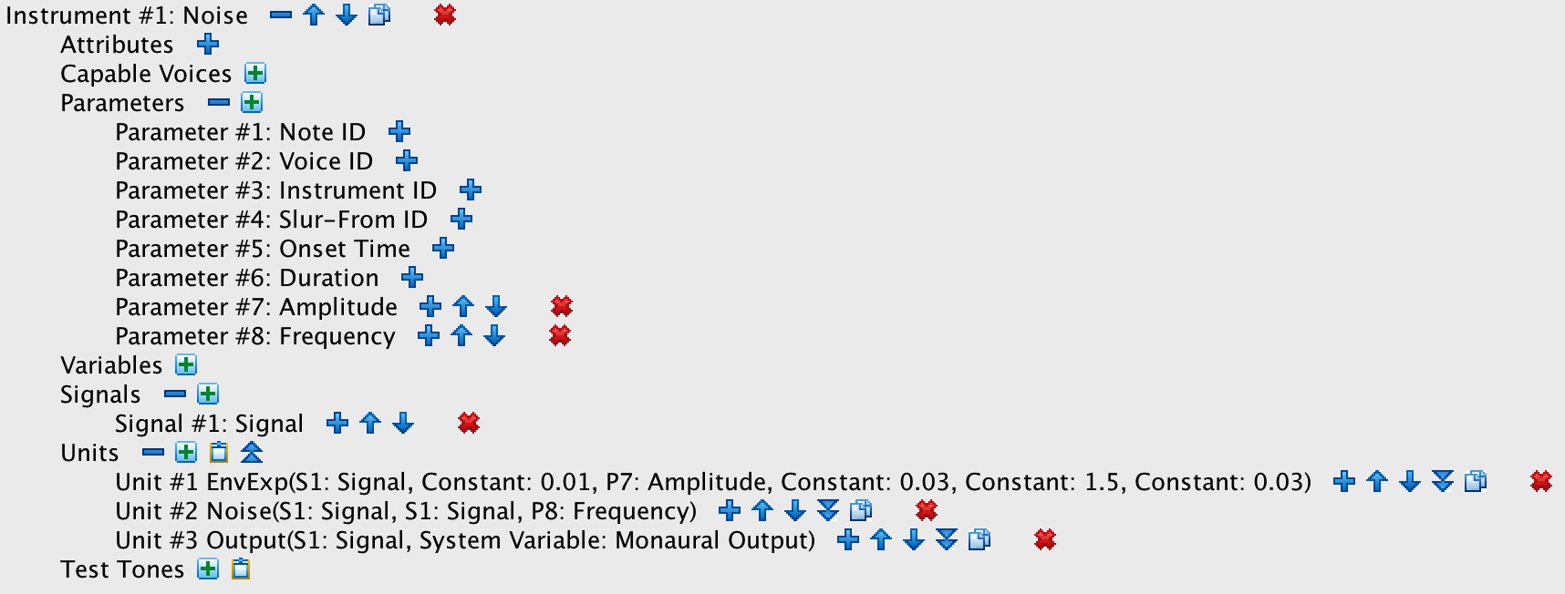
| Figure 6-1: Enveloped noise instrument with explicit signal multiplication. | Figure 6-2: Enveloped noise instrument with implicit signal multiplication. |
Video 1-1 animates how a Multiply unit imposes an envelope (the Multiplier) upon an audio signal (the Multiplicand). The left-side stage labeled Oscillator looks up samples from a stored waveform. The vertical scale gives the intensity of the signal, while the horizontal scale of the waveform is 10 pixels per sample. The right-side stage labeled Output is a signal queue. It carries through the Oscillator's vertical scale, but reduces the horizontal scale to one pixel per sample. Each frame of the animation scrolls the Output contents rightwards by one pixel, allowing the newly generated sample to be plotted in the leftmost position. The samples thus plotted proceed from newer samples on the left to older samples on the right, reversing theorder of presentation normally expected a time-series graph.
800 samples are generated over the course of each video. Since the Output queue only has room for 640 samples, the earliest 160 samples have fallen off the right side of the queue when the video is done.
The operation of the Oscillator stage is indicated by the arrow which first extends vertically from the
the x-axis to the waveform value and which continues horizontally over to the
Output queue. The starting point of this arrow indicates the current Phase
value, which wraps around from 0 (inclusive) on the left to 16 (exclusive) on the right.
The sampling increment for Video 1-1 is 0.0618, which means that the vertical portion of the
Oscillator-to-Output arrow advances rightward at a rate of 0.0618×10=0.618
pixels per frame. The number of frames required to complete one oscillation is 16/0.0618=258.9, which means that Phase
will cycle from 0 to 16 800/258.9=3.1 times over the duration of the video. The Phase will linger
over each Index for 1/0.0618=16.2 samples, so the Output
wave proceeds as a series of horizontal steps, each 16 (sometimes 17) samples wide.
Video 1: An oscillating audio signal (Multiplicand) multiplied by an envelope control signal (Multiplier).
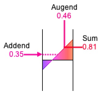
Figure 7: Addition y = x + b
rendered with x = 0.46 and b = 0.35.
Orientation: input-top/output-right.
Addition (Mixing)
Consider addition. Addition produces an output from two inputs. The primary input is called the augend, the secondary input is called the addend, and the output is called the sum. If x represents the augend, b represents the addend, and y represents the sum, then the transformation can be rendered by graphing y = x + b, which is a straight line with a slope of 45%, crossing the y-axis at b.
The Add unit implements the operation
Output(K) = Input1(K) + Input2(K),
where
-
Output(K), the sum, is theKth sample of the output signal, -
Input1(K), the augend, is theKth sample of the primary input signal, and -
Input2(K), the addend, is theKth sample of the secondary input signal.
Video 2-1 animates how signals mixed together by adding their corresponding samples.
Video 2-1: Sine waveforms generated by sweeping a radius around a circle.
Video 2-2 animates how signals mixed together by adding their corresponding samples.
Video 2-2: Sine waveforms generated by sweeping a radius around a circle.
Audio to Control
You can transform a noise signal ranging from -1 to 1 into a randomized control signal ranging from 0 to 1 by multiplying the signal by 0.5, then adding 1.
Channel Balance
Amplitude Envelopes
Recall the discussion of the “simplest instrument”, which directed a signal from an Oscillator directly to an Output channel. Having an instantaneous attack and an instantaneous release, the “simplest” design produces sounds which begin and end with clicks.
The present entry
My Sound engine implements three envelope flavors: sustained, exponential, and AHDSR. However more dynamic envelopes may be derived by
Linear Ramps
Linear ramps change by equal increments over equal time durations. In particular for the very short duration separating two consecutive samples there is a corresponding increment, also very small, that can be added to the previous sample to obtain the current one. The rate of change over a one second duration is the slope of the ramp.
The Line unit implements the operation
Output(K) = Output(K-1) + δ,
where
-
N, the number of samples, is calculated by multiplying the duration in seconds by the sampling rate. -
Output(0), the origin, is the starting value of the segment, -
Output(N), the goal (never actually reached), is the ending value of the segment, -
Output(K), the new augend, is theKth sample of the output signal, -
Output(K-1), the old augend, is theK-1th sample of the output signal, and -
δ, a constant addend, is calculated as(Output(N)-Output(0))/N.
The Line unit acts effectively as a numerical integrator, which is a fancy way to say ‘running sum’.2
Exponential Ramps
Exponential ramps change by equal ratios over equal time durations. In particular for the very short duration separating two consecutive samples there is a corresponding ratio, also very small, that can be multiplied with the previous sample to obtain the current one. Exponential ramps are always positive. When the ramp asends, the ratio over one second is the growth rate. When the ramp descends, the ratio over one second is the decay rate.
The Growth unit implements the operation
Output(K) = Output(K-1) × μ,
where
-
N, the number of samples, is calculated by multiplying the duration in seconds by the sampling rate. -
Output(0), the origin, is the starting value of the segment, -
Output(N), the goal (never actually reached), is the ending value of the segment, -
Output(K), the new multiplicand, is theKth sample of the output signal, -
Output(K-1), the old multiplicand, is theK-1th sample of the output signal, and -
μ, a constant multiplier, is calculated as theNth root ofOutput(N)/Output(0).
The Growth unit acts effectively as a running product. The result is the same as if one
-
Initialized a running sum
S(0) = log(Output(0)), -
Calculated a constant addend
δ = log(μ) = (log(Output(N)) - log(Output(0)))) / N, -
Returned
Output(K) = exp(S(K)), whereS(K) = S(K-1)+δ.
Frequency Modulation
Operation of the Digital Filter
Operation of the RMS Unit
Comments
- MIDI files are an example of a digital signal within which the time interval separating consecutive events is variable.
- It would have happened during the spring semester of 1979: One day in our computer sound-synthesis class at UB, mathematician John Myhill took on the task of explaining John Chowning's method of synthesizing complex tones by frequency modulation. While describing how a variable frequency input affects the behavior of a digital oscillator, Myhill characterized the oscillator's frequency input as “an integrator”.
| © Charles Ames | Page created: 2013-02-20 | Last updated: 2017-06-24 |