Cascaded Digital Filters

Overview

This page investigates what happens when two or more digital filters are used in combination. There are two ways of combining filters: in parallel or in cascade.

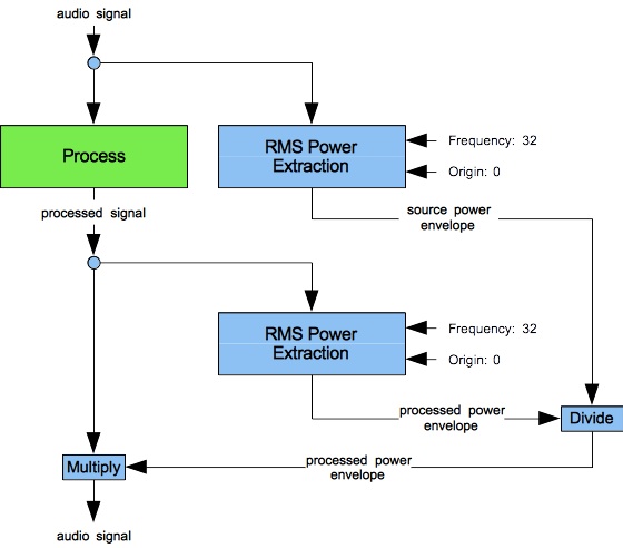
Figure 1: Design for sound-synthesis instruments using RMS power extraction to mitigate filter gain.

Combining filters in parallel means feeding the same source input into two or filters, and then mixing (adding) the separate filter outputs together. Although Klatt, 1980 advocated parallel filtering for synthesizing fricative consonants, Klatt did not supply frequency data with which would allow his approach to be replicated. I have nothing more to write about parallel filtering.
Combining filters in cascade means treating two or more filters as a sequence in which the output of one filter becomes the input for the next filter. This approach is heavily favored in the sound-synthesis literature.

One of the main challenges posed by digital filtering is that signal amplitudes coming out of a digital filter vary widely from amplitudes going in. The quotient of output amplitude divided by input amplitude is known as the gain. Gains from digital filtering tend to be much lower than unity, but the opposite can also be true, especially when inbound frequencies align with resonant peaks.

Figure 1 presents the design pattern used throughout this page (and elsewhere) to moderate gain from digital filtering. I learned both the design and the underlying procedure for RMS power extraction at Barry Vercoe's 1978 summer computer sound-synthesis workshop. The green box labeled “Process” represents a bank of one or more digitals filters, examples of which will be considered through the remainder of this page. The basic idea is to normalize the output signal by dividing the raw result by its RMS power. The RMS envelope of the input signal may then be restored.

Low-Pass Filtering

In the The Audio Programming Book, Victor Lazzarini presents the difference coefficients used by FilterLowPass2B as part of a suite of 2nd-order “Butterworth” filters. According to Wikipedia, Butterworth filters are characterized by flat frequency response in the “pass band”, rapid drop-off at the cutoff frequency, and low signal leakage in the “stopped band”.


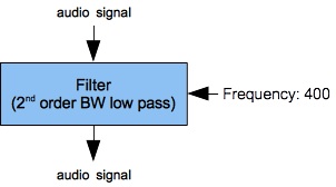
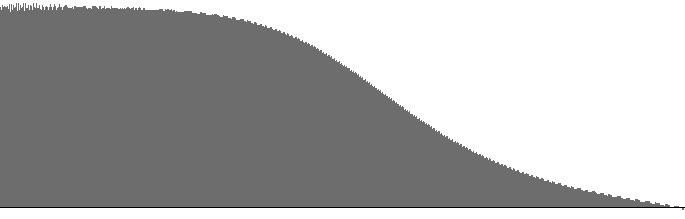
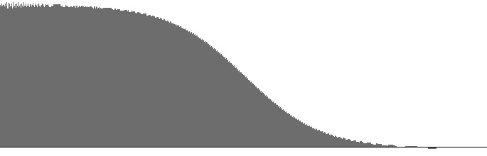
Figure 2 (a): Single low-pass filter.	Figure 2 (b): Amplitude versus log(frequency) with 400 Hz. “cutoff” for the filter shown in Figure 2 (a).	Figure 2 (c): Log(amplitude) versus log(frequency) with 400 Hz. “cutoff” for the filter shown in Figure 2 (a).

Figure 2 (a) shows a filter bank consisting of a single FilterLowPass2B unit. This unit implements Lazzarini's 2nd-order Butterworth low-pass filter with a 400 Hz. cutoff frequency. The frequency reponse curves for this filter with a 400 Hz. cutoff are replotted in Figure 2 (a) and Figure 2 (b). A set of frequency-response curves for various cutoff frequencies appears elsewhere; however, the 0 dB threshold in Figure 2 (c) has been decreased to reveal a severe downward bend up near the Nyquist limit.

The dropoff rate during the long sloping region of Figure 2 (c) is -2.9 dB/octave. This drop-off rate is hardly rapid. If you have an expert like Lazzarini on call, such an expert would but better results may be achieved by higher-order filters .


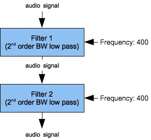
Figure 3 (a): Two low-pass filters in cascade.	Figure 3 (b): Amplitude versus log(frequency) with 400 Hz. “cutoff” for the filter bank shown in Figure 3 (a).	Figure 3 (c): Log(amplitude) versus log(frequency) with 400 Hz. “cutoff” for the filter bank shown in Figure 3 (a).

Alternatively, one can cascade two or more 2nd-order low-pass filters to obtain a 4th order result. The filter bank shown in Figure 3 (a) shows a filter bank cascading two FilterLowPass2B units sharing a common 400 Hz. cutoff frequency. Figure 3 (b) and Figure 3 (c) plot the frequency-response curves resulting from this cascade. The dropoff rate during the long sloping region of Figure 3 (c) is -6.9 dB/octave. This compares very favorably with a single 2nd-order filter if your objective is to suppress all frequencies in the stopped band.

Dual Resonances

The 2nd Order Butterworth Band-Pass Filter page demonstrated that the FilterBandPass2B unit produces beautifully symmetric resonance peaks. By contrast, the 2nd Order Band-Pass Filter page revealed that FilterBandPass2 unit originally implemented as FLT in MUSICV suppresses high frequencies more severely while leaking prodigiously in the low-frequency stop band. One would be tempted to deprecate FLT. I want to demonstrate, both here and under the next heading, that the old FLT unit still has its uses.


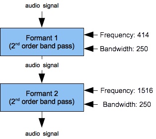
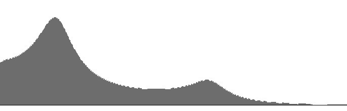
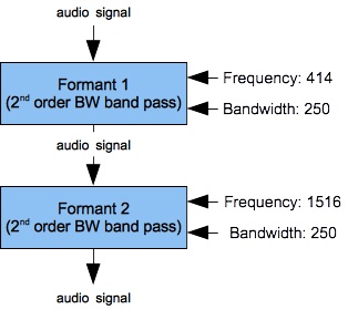
Figure 4 (a): Two cascaded FilterLowPass2 units with resonance peaks at 414 Hz. and 1516 Hz.	Figure 4 (b): Amplitude versus frequency for the filter bank shown in Figure 4 (a)	Figure 4 (c): Log(amplitude) versus frequency for the filter bank shown in Figure 4 (a)

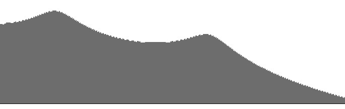
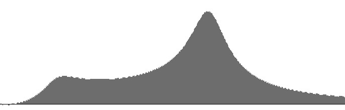
Figure 5 (a): Two cascaded FilterLowPass2B units with resonance peaks at 414 Hz. and 1516 Hz.	Figure 5 (b): Amplitude versus frequency for the filter bank shown in Figure 5 (a)	Figure 5 (c): Log(amplitude) versus frequency for the filter bank shown in Figure 5 (a)

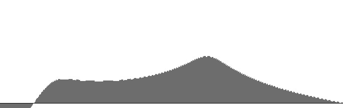
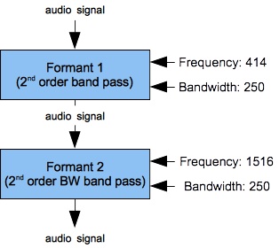
Figure 6 (a): A FilterLowPass2B unit with resonance peak at 414 Hz. cascaded into a FilterLowPass2 unit with resonance peak at 1516 Hz.	Figure 6 (b): Amplitude versus frequency for the filter bank shown in Figure 6 (a)	Figure 6 (c): Log(amplitude) versus frequency for the filter bank shown in Figure 6 (a)

Figures 4 (a) through 6 (b) plot frequency responses for various pairings of FilterLowPass2 (FLT) and FilterLowPass2B (Butterworth) band-pass filters. Each frequency-response curve is plotted along a direct (non-logarithmic) frequency scale ranging from 16 to 2000 Hz. The (b) graphs are independently scaled, while the (c) graphs share a common scale. The resonance peaks correspond with the two lowest formants of the neutral vowel, or “schwa” (ə). Both peaks have 250 Hz. bandwidths.

The 1516 Hz. peak is very strongly attenuated in Figure 4 (a-b). This explains why in my own early attempts to synthesize vowels, the long E sound — with lower resonance peaks at 227 and 2208 Hz. — went faint. Among speech synthesis sources I have consulted, Klatt, 1980 suggests that resonant peaks should decrease in gain as peak frequency increases. Klatt further asserts that:

The advantage of the cascade connection is that the relative amplitudes of formant peaks for vowels come out just right (Fant, 1956) without the need for individual amplitude controls for each formant.

Klatt's speech synthesizer produced vowels by cascading five resonators, each equivalent to the Sound engine's FilterLowPass2 unit. He lists the peak frequency for resonator #5 as 3750 Hz. However the results in Figures 4 (a-b) lead me to wonder whether Klatt's uppermost vowel formants were in any way audible.

Likewise the 414 Hz. peak is too strongly attenuated in Figures 5 (a-b). This happens because the FilterLowPass2B unit suppresses the lower stopped-band frequencies much more effectively than the FilterLowPass2 unit does.

Figure 6 (a-b) produces resonances of equal gain. This is ideal. Remember that the actual generated spectrum will only have uniform peaks if the source signal is itself uniform — for examples, white noise or a pulse waveform with equal-amplitude harmonics.

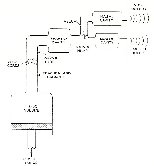
Figure 7: Functional components of the vocal tract. From Flanagan, 1972, page 24.

Emulating Oral Resonances

Figure 7 shows the functional components of the vocal tract.

Sound energy provided by the lungs is converted into tone or aspirate noise (whisper) in the larynx, from which point the sound is processed by the vocal tract.
The vocal tract processes sound in one of two modes depending on whether the sound ultimately eminates from the lips or from the nose. You don't get sounds from both outputs at once so any attempt to emulate vocal resonance needs the ability to switch between modes.
Normal emination is through the lips. In this mode there are three sources of resonance: the pharanx, the mouth, and the lips themselves. Each resonance appears in the frequency-response curve as a peak; that is, as a region of frequency enhancement. Frequency-response resonance peaks are known among phoneticists as formants.
Alternate emination is through the nose. This second mode is considered below.

Our present goal is to assemble a filter bank which emulates how sounds are transformed by resonances in the pharynx, in the mouth cavity, and through the lips. The dual-filter banks considered under the previous heading implemented a low-frequency resonance corresponding to the lips and a mid-range resonance corresponding to the pharynx. Two resonances are sufficient to distinguish common vowels; however, liquid consonants such as r and l require the mouth cavity to be accomodated as a third, higher resonance. For that reason it is worthwile to investigate combinations of three band-pass filters.


Figure 8 (a): A pair of FilterLowPass2B units cascaded into FilterLowPass2.	Figure 8 (b): Amplitude versus frequency for the filter bank shown in Figure 8 (a) with resonance peaks determined by the schwa vowel (`ə`): F1=414, F2=1516, and F3=2500.	Figure 8 (c): Log(amplitude) versus frequency for the filter bank shown in Figure 8 (a) with resonance peaks determined by the schwa vowel (`ə`): F1=414, F2=1516, and F3=2500.

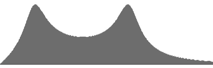
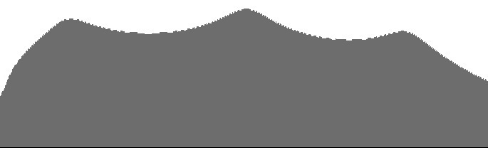
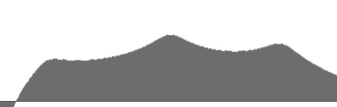
Figures 8 (a-b) show frequency-response curves obtained when a pair of two FilterLowPass2B (Butterworth) units cascades into a single FilterLowPass2 (FLT) unit. Frequences range directly (non-logarithmically) along the horizontal axis from 16 to 3000 Hz. As in Figure 6 (a-b), cascading two Butterworth filters causes the mid-frequency resonance to strongly attenuate the low-frequency resonance.


Figure 9 (a): A FilterLowPass2B unit cascaded into a pair of FilterLowPass2 units: amplitude versus frequency.	Figure 9 (b): Amplitude versus frequency for the filter bank shown in Figure 9 (a) with resonance peaks determined by the schwa vowel (`ə`): F1=414, F2=1516, and F3=2500.	Figure 9 (c): Log(amplitude) versus frequency for the filter bank shown in Figure 9 (a) with resonance peaks determined by the schwa vowel (`ə`): F1=414, F2=1516, and F3=2500.

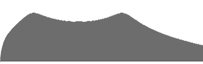
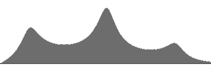
The frequency-response curves in Figures 9 (b-c) doesn't exactly produce uniform peaks, but the peaks are much more uniform than in Figures 8 (b-c). Remember that the ear perceives loudness logarithmically, so it is the (c) graphs that really matter, and in Figure 9 (c) the peaks look nearly the same.

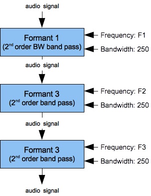
After considering these two alternatives, it seems that the combination of one Butterworth unit with two FLT units offers the most promising results for speech synthesis.

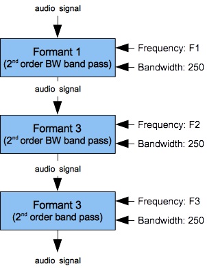
The low-frequency resonator identified as “Formant 1” in Figure 9 (a) corresponds to the lips when they are open and to the nose when emination through the lips is closed. The control frequency of this lowest resonator is traditionally designated F₁ (for formant #1).
The middle-frequency resonator identified as “Formant 2” in Figure 9 (a) corresponds to the pharanx. The control frequency of this middle resonator is traditionally designated F₂ (for formant #2).
The higher-frequency resonator identified as “Formant 3” in Figure 9 (a) corresponds to the mouth cavity. The control frequency of this high resonator is traditionally designated F₃ (for formant #3).

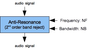
Taming the Notch Filter

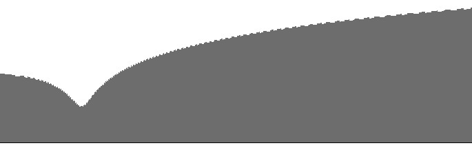
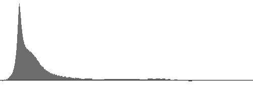
Another page on this site, 2nd Order Band-Reject Filter, explored a filter design from Julius Smith that suppressed frequencies very effectively in a narrow range around a specified “notch” frequency, so long as the bandwidth was set not much greater than 100 Hz. Figures 10 (a-c) show the frequency response for a FilterBandReject2 with the notch frequency set to 440 Hz. and the bandwidth set to 25 Hz. These graphs are plotted along a direct (non-logarithmic) frequency scale ranging from 16 to 2500 Hz.


Figure 10 (a): A single FilterBandReject2 unit.	Figure 10 (b): Amplitude versus frequency for the filter shown in Figure 10 (a) with NF=440 and NB=25.	Figure 10 (c): Log(amplitude) versus frequency for the filter shown in Figure 10 (a) with NF=440 and NB=25.

Notch filtering is essential for the synthesis of nasal consonants, fricative consonants, and for muting effects. However as Figures 10 (a-c) demonstrate, frequency responses under Smith's design increase exponentially above the notch. This is a very serious downside; however, the problem can be mitigated by low-pass filtering.


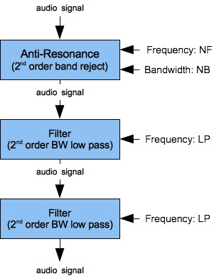
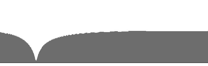
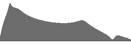
Figure 11 (a): A FilterBandReject2 unit cascaded into a pair of FilterLowPass2B units with slaved cutoff frequencies.	Figure 11 (b): Amplitude versus frequency for the filter shown in Figure 11 (a) with NF=440, NB=25, and LP=550.	Figure 11 (c): Log(amplitude) versus frequency for the filter shown in Figure 11 (a) with NF=440, NB=25, and LP=550.

I found that single 2nd-order low-pass filter could not accomodate the gain from a notch filter. However, if I cascaded the notch filter into a pair of 2nd-order low-pass filters I could induce a flat upper-pass-band response. Figures 10 (a-c) show the results of my investigation. As with Figures 10 (b-c), the graphs in Figures 11 (b-c) are plotted along a direct (non-logarithmic) frequency scale ranging from 16 to 2500 Hz. The low-pass cutoff of 550 Hz. was selected by trial and error. Raising the cutoff much above 550 Hz. causes the upper-pass-band response to trend upwards.

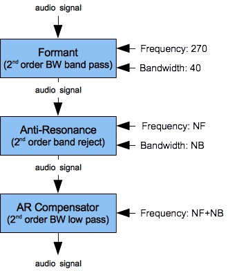
Figure 2: Filter-bank extension with low-frequency formant and antiresonance, plus a low-pass filter to compensate for the antiresonator's high-frequency gain.

Emulating Nasal Resonances and Anti-Resonances

Remember from Figure 7 that the vocal tract produces sound in two modes, one eminating from the lips and the other eminating through the nose. The first mode was considered previously. In nasal mode the pharanx and mouth provide resonance, but emination through the lips is closed. However the nasal cavity itself contributes fixed resonances at 270 Hz. and 480 Hz.

Nasal sounds are also characterized by anti-resonances. These appear in the frequency-response curve as a trough; that is, as a region of frequency suppression.

Some writers attribute anti-resonances to sinuses, and this seems plausible in secondary instances.
However, it seems very unlikely that the most conspicuous anti-resonance is due to sinuses. Sinuses do not change. By contrast, the primary anti-resonance varies from low for m through mid-range for n to high for ŋ. This explains why most writers concur with Flanagan, 1977's assertion that the “The blocked oral cavity acts as a side branch resonator” (p. 77).

Our goal is to emulate how sounds are transformed by passage through the pharyx and the nasal cavity. This will be accomplished by cascading two banks of filters.

The first filter bank is the one developed for vowels and liquids, previously shown in Figure 9 (a). Since nasal sounds do not employ the lips, the lowest resonance F₁ may be co-opted by the nasal cavity's upper (480 Hz.) fixed resonance.
The second filter bank, shown in Figure 12, imposes the low resonance with peak frequency F₀ — this value remains fixed at 270 Hz. It also includes the primary antiresonance and a 2nd-order low-pass filter acting as “AR Compensator”. Why not two low-pass filters after the trouble taken under Taming the Notch Filter? Well, the low fixed resonance is also a 2nd order filter. The notch frequency for this second filter bank is designated in Figure 12 as NF, while the bandwidth is designated as NB.


Figure 13 (a): Amplitude versus frequency for the bilabial nasal `m`. F₀=270, F₁=450, F₂=1270, and F₃=2130, NF=450, and NB=25.	Figure 13 (b): Log(amplitude) versus frequency for the bilabial nasal `m`. F₀=270, F₁=450, F₂=1270, and F₃=2130, NF=450, and NB=25.

Figure 14 (a): Amplitude versus frequency for the alveolar nasal `n`. F₀=270, F₁=450, F₂=1340, and F₃=2470, NF=1200, and NB=75.	Figure 14 (b): Log(amplitude) versus frequency for the alveolar nasal `n`. F₀=270, F₁=450, F₂=1340, and F₃=2470, NF=1200, and NB=75.

Figure 15 (a): Amplitude versus frequency for the velar nasal `ŋ`. F₀=270, F₁=450, F₂=2208, and F₃=3079, NF=3000, and NB=100.	Figure 15 (b): Log(amplitude) versus frequency for the velar nasal `ŋ`. F₀=270, F₁=450, F₂=2208, and F₃=3079, NF=3000, and NB=100.

Figures 13 (a) through 15 (b) plot frequency-response curves for the nasal sounds m, n, and ŋ. Frequences range directly (non-logarithmically) along the horizontal axis from 16 to 3500 Hz. The (a) graphs are vertically scaled to fit the largest response magnitude, while the (b) graphs share a common vertical scale.

The NF values come from Felicity Cox, while the NB values come from trial and error. The F₀, F₁, F₂, and F₃ values for m, n come from Klatt, 1980. Cox agrees with Klatt on F₀ and F₁ but suggests that F₂ and F₃ should be influenced by surrounding vowels. This makes sense (compare the m sounds in “me” and “moo”) but Klatt's static values proved more convincing. Unfortunately, Klatt's table III contains entries only for m and n — not ŋ. I made an educated guess and employed the F₂ and F₃ from i (as in “see”) from the table of vowels. This choice seems to work for ŋ.

The prominance of the F₀ peak in the (a) figures is consistent with Felicity Cox's observation that F₀ (which she designates N1) be of “of high intensity compared with the rest of the spectrum”.

Page created: 2014-02-20

Last updated: 2015-07-12