Statistical Feedback
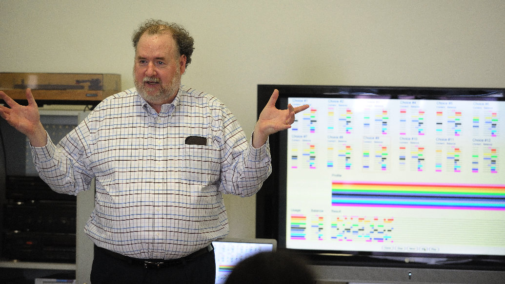
Presenting statistical feedback at the 2011 Ostrava Days Institute. Credit: Ostrava Center for New Music — Martin Popelar.
Overview
Statistical Feedback is the name I use for a decision-making method which actively promotes balance among resources. This method is heuristic rather than algorithmic — a distinction I explain further in my 1992 article, “Quantifying Musical Merit”. It operates on a fair-share principle, that is, the resources falling most behind their fair share of usage receive first consideration going forward.
The trail of discovery that led me to statistical feedback is recounted in a 1990 Perspectives of New Music article, “Statistics and Compositional Balance”. That article describes what I now call the special method, which chooses among single items. Subsequently there evolved a general method, which employed the minimax principle to select among groups of items. The general method was originally described in “Quantifying Musical Merit”. The present demonstration applet employs this general method. There is also a third method called the balanced-bit generator; this third method is demonstrated elsewhere on this site.
The graphic demonstration described here was first presented in a non-web implementation at the
Ostrava New Music Days Institute in August, 2011.
The applet version posted on this site in 2013 included the three original demonstration examples plus two new offerings.
These were provided as downloadable XML files which could be
run using the applet. The applet also provided a graphical editor, allowing you to design scenarios of your own. (For more details, see the
Instructions page.) Since the powers that be on the internet have now abandoned applet
technology, the present (2017) update of this page offers MP4
animations of the selection process and MP3 sound examples
of generated results. The latter were converted from applet-generated MIDI files
at www.online-convert.com.
The graphical editor instructions expose four component types: Chromas, Sounds, Chords, and Events. Each Chord references one or more Sounds, and each Sound references a single Chroma. (My usage of the word “chroma” here follows that of James Tenney in Meta+Hodos.) The collection of Events comprises a sequence, where the duration of one Event determines the starting time of the succeeding Event. The applet animates the process of selecting a Chord for each Event.
Expressed in the jargon of my production framework,
- The Event sequence is a problem implemented using a “Beauty Contest” strategy (heuristic selection without backtracking). Events are processed in time order, proceeding strictly from left to right.
- Individual Events stand as decisions, the options of which are Chords. The method of chord-selection is heuristic, guided by statistical feedback.
- The “general” method of statistical feedback is incorporated into the production framework. Within the framework, the options available to a decision can have multiple values, but each value maps to a single state. Each state identifies a resource for statistical feedback to keep in balance. Option values in the framework correspond to Sounds in the present applet, while states correspond to Chromas.
Four of the five examples described below promote balance directly between Sounds, and this is accomplished by creating one-to-one associations between Sounds and Chromas. However in Example #5 the Sounds stand for pitches while the Chromas stand for scale degrees.
Example #1: Simple Uniform Selection
Example #1 balances the three Chroma, Sound, Chord triplets detailed in Table 2.
| Index | Color | Percussion | MIDI Program | MIDI Key | MIDI Velocity |
| 0 | Black | false | OBOE | C5 | 90 |
| 1 | Blue | false | MARIMBA | C#3 | 90 |
| 2 | Cyan | false | BASSOON | B2 | 90 |
Table 2: Sounds of
Feedback-Uniform.xml.
All three components in the same triplet share a common index. Thus Chord #0 contains Sound #0, which references Chroma #0. The weight contour for each Chroma maintains the value 1.0 statically over the duration of the example. Combining the three contours together yields the profile shown in Figure 1. The example spans 90 Events, each lasting one unit (i.e. one quarter note).
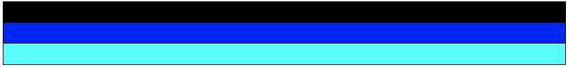
Figure 1: Profile of theFeedback-Uniform.xmlexample.
You can witness the selection process for Example #1 by playing the following animation. Before you do that, you should first understand the components of the image. These components arranged in three rows:
- The first row presents the collection of chords available for selection. Each Chord has one bar graph showing the Content of sounds within the chord alongside second bar graph predicting the chromatic Balance; that is, how chroma usages will deviate around their center points.
- The second row is a Profile showing how the weight of each sound evolves over time. For Example #1, this is the same information given in Figure 1.
- The third row begins with two bar graphs. The first bar graph in row 3 shows the relative chromatic Usage up to the current moment of selection. The second bar graph in row 3 shows the actual chromatic Balance, again as deviations around their center point. The third component in row 3 is a grid plotting which chromas have been selected so far for each of the 90 events.
|
|
|
|
|
|
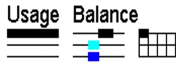
To understand how row 3's Usage and Balance graphs work, refer to Figure 2 (a). This figure assumes that the first decision has already been made, and that the first decision selected Sound #0 for Event #1.
- The Usage graph contains a full black bar in the uppermost position, reflecting the fact that only Sound #0 has been selected so far.
- The Balance graph shows a black bar extending right from the center point, reflecting the fact that Sound #0 has advanced beyond its fair share of usage.
- The Usage graph also shows blue and cyan bars extending left from the center point. These reflect the facts that Sound #1 and Sound #2 have each fallen behind their fair shares of usage.
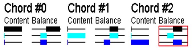
To understand how the Content and Balance graphs work for each chord in row 1, refer to Figure 2 (b).
- The Content graph for Chord #0 contains a full black bar in the uppermost position, reflecting the fact that Chord #0 employs only Sound #0.
- The Balance graph for Chord #0 predicts what that Balance graph down in row 3 will come to look like in the circumstance that Chord #0 is selected for Event #2.
The goal of statistical feedback is select the option (for this purpose a chord) which gives each resource (for this purpose a sound) its fair share of usage. This situation is achieved graphically when the values in row 3's Balance graph cluster most tightly around the center point.
- Consider selecting Chord #0 for Event #2. This would advance Sound #0 while allowing Sound #1 and Sound #2 to fall even farther behind.
- Alternatively, consider selecting Chord #1 for Event #2. This would enable Sound #1 to catch up with Sound #0 while neglecting Sound #2.
- The remaining alternative, Chord #2, would enable Sound #2 to catch up with Sound #0 while neglecting Sound #1.
Neither Chord #1 nor Chord #2 achieves perfect balance, but either option is superior to Chord #0. Which to use?
This is where heterogeneity comes into play. Small random values added into the values shown by the chordal Balance graphs tip the balance whenever it teeters on the knife edge. Thus while Chord #1 and Chord #2 seem equally preferable in Figure 2 (b), randomness tips the balance in favor of Chord #2. Whose selection is indicated by the red rectangle.
Go ahead and play the video now. In the event that your browser does not support my video formats, I present the composed
result in Figure 3 (a).
Feedback-Uniform.mp3 provides an audio realization of the generated result.
A second result, generated using a different random seed, appears as
Figure 3 (b).

Figure 3 (a): TheFeedback-Uniform.xmlexample, realized with Heterogenity=0.1 and Seed=0.

Figure 3 (b): TheFeedback-Uniform.xmlexample, realized with Heterogenity=0.1 and Seed=1.
Figure 3 (a) and Figure 3 (b) illustrate the behavior properly expected when the weights are uniformly static, when all Events have the same duration, and when the Heterogenity attribute is small. Notice that the first three Events, among themselves, utilize all three Sounds. Likewise, the fourth, fifth, and sixth Events, among themselves, utilize all three Sounds. So it goes for entire sequence of events.
This is the same behavior one would expect from the SERIES feature of
Gottfried Michael König's
Project 2 program.
Thus are confirmed the antecedents of statistical feedback in European post-serial aleatoric methods.
Later examples will demonstrate how statistical feedback responds to changing durations, and to non-uniform balances. However the current example presents the best opportunity to illustrate what happens when the Heterogenity attribute is substantially greater than unity. Figure 3 (c) shows a result obtained with the Heterogenity jacked up to 10. Notice that the result sometimes lingers on one specific Sound for three or more successive Events, or elsewhere that the result emphasizes two Sounds to the exclusion of the third. The Balance graph after the final decision is certainly out of kilter. Yet the Usage graph demonstrate that over the result as a whole, the proportions of Events allocated to the three different Sounds agree very closely.

Figure 3 (c): TheFeedback-Uniform.xmlexample, realized with Heterogenity=10 and Seed=2.
Example #2: Chromatic Chords with Variable Durations
This example demonstrates how statistical feedback accomodates selection at a group level with changing event durations. Here, selecting a chord for a single Event having a duration of two units affects balances in the same way as selecting the same chord for two Events, each having durations of one unit.
Example #3 employs twelve Sounds, each paired with a Chroma that shares the same index. The sounds represent all twelve degrees of the chromatic scale. Although Table 3 lists the pitches in circle-of-fifths order, this has the effect of distributing pitches which are close on the circle of fifths over disparate registers.
| Index | Color | Percussion | MIDI Program | MIDI Key | MIDI Velocity |
| 0 | Pink | false | BASS_ACOUSTIC | C2 | 90 |
| 1 | Red | false | CELESTA | G3 | 90 |
| 2 | Orange | false | CLARINET | D4 | 90 |
| 3 | Yellow | false | OBOE | A5 | 90 |
| 4 | Green | false | CELLO | E2 | 90 |
| 5 | Gray | false | BASSOON | B3 | 90 |
| 6 | Black | false | HARP | F#4 | 90 |
| 7 | Dark Gray | false | VIBRAPHONE | C#5 | 90 |
| 8 | Light Gray | false | PIANO_ACOUSTIC_GRAND | A!2 | 90 |
| 9 | Cyan | false | FRENCH_HORN | E!3 | 90 |
| 10 | Blue | false | TRUMPET | B!4 | 90 |
| 11 | Magenta | false | MARIMBA | F5 | 90 |
Table 3: Sounds of Example #2.
Like Example #1, the weight contour for each Chroma maintains the value 1.0 statically over the duration of the example. However, the present Example #2 exploits all twelve Chromas. Combining the twelve contours together yields the profile shown in Figure 4.
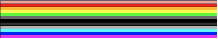
Figure 4: Profile of theFeedback-Chromatic.xmlexample.
Example #2 contains 64 events mixing durations of 1, 2, and 3 units. To determine the sequence of durations, I wrote a small Java program that employed statistical feedback with low heterogeneity. This program accorded unit weight to durations of 1 unit, weight 1/2 to durations of 2 units, and weight 1/3 to durations of 3 units. The result had two features:
- Total amount of time filled by any one duration type was approximately 1/3 the total duration of the example.
- The longer duration types had roughly equal spacing among the sorter duration types.
There are twelve Chords. Each Chord contains four Sound values, chosen to favor dissonant sonorities. Each Sound appears in four Chords; thus the Chord collection gives equal representation to each of the twelve chromatic degrees, which is consistent with the weights graphed in Figure 4. Such consistency helps the decision engine select suitable Chords, but it is no means required.
| Choice Index | Value 0 | Value 1 | Value 2 | Value 3 | Value 4 | Value 5 | Value 6 | Value 7 | Value 8 | Value 9 | Value 10 | Value 11 |
| 0 | 0 | 1 | 6 | 10 | ||||||||
| 1 | 0 | 2 | 3 | 9 | ||||||||
| 2 | 0 | 4 | 7 | 8 | ||||||||
| 3 | 0 | 1 | 5 | 11 | ||||||||
| 4 | 1 | 2 | 6 | 9 | ||||||||
| 5 | 3 | 4 | 5 | 7 | ||||||||
| 6 | 3 | 6 | 7 | 11 | ||||||||
| 7 | 2 | 8 | 9 | 10 | ||||||||
| 8 | 3 | 4 | 5 | 10 | ||||||||
| 9 | 1 | 5 | 6 | 8 | ||||||||
| 10 | 2 | 8 | 9 | 11 | ||||||||
| 11 | 4 | 7 | 10 | 11 |
Table 4: Chords in Example #2.
You can witness the selection process for Example #2 by playing the following animation.
In the event that your browser does not support my video formats, I present the composed
result in Figure 5.
Feedback-Chromatic.mp3 provides an audio realization of the generated result.
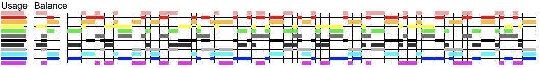
Figure 5: TheFeedback-Chromatic.xmlexample, realized with Heterogenity=0.01 and Seed=0.
Look at the Usage graph. Selecting among groups of Sounds posed a challenge, since Chords could potentially mix over-used Sounds with under-used Sounds. Selecting for Events with longer durations posed a second challenge, since longer durations affect balances more radically. Yet despite these challanges the bars in the Usage graph come out remarkably even.
Example #3: Linear Evolution
Example #3 demonstrates how statistical feedback copes with evolving weights. For this example I have chosen to employ percussion sounds. There are five Sounds, each paired with a Chroma that shares the same index.
| Index | Color | Percussion | MIDI Key | MIDI Velocity |
| 0 | Yellow | true | CYMBAL_RIDE1 | 90 |
| 1 | Magenta | true | SNARE_DRUM1 | 90 |
| 2 | Cyan | true | TOM_HIGH1 | 90 |
| 3 | Blue | true | TOM_LOW1 | 90 |
| 4 | Black | true | BASS_DRUM1 | 90 |
Table 5: Sounds of Example #3.
The weight contour for the cymbal (Sound #0) holds at unity for the duration of the example. This does not mean that the cymbal participates in every event. I'll explain why after we see the results. The weight contours for the tom-toms (Sound #2 and Sound #3) both start at unity, but both ramp down to zero over the duration of the example. Tom-tom activity is complemented by snare (Sound #1) and bass-drum Sound #4 activity. The weight contours for these latter sounds begins at zero and ramps up to unity. All these contours join together into the profile shown in Figure 6.
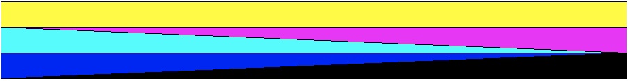
Figure 6: Profile of the
Feedback-Evolution.xml example.
There are eight Chords. Chords 0-3 are single Sounds not including cymbal strikes. Chords 4-7 are double Sounds including cymbal strikes.
| Chord Index | Sound Index | Color | MIDI Key |
| 0 | 1 | Magenta | SNARE_DRUM1 |
| 1 | 2 | Cyan | TOM_HIGH1 |
| 2 | 3 | Blue | TOM_LOW1 |
| 3 | 4 | Black | BASS_DRUM1 |
| 4 | 0 | Yellow | CYMBAL_RIDE1 |
| 1 | Magenta | SNARE_DRUM1 | |
| 5 | 0 | Yellow | CYMBAL_RIDE1 |
| 2 | Cyan | TOM_HIGH1 | |
| 6 | 0 | Yellow | CYMBAL_RIDE1 |
| 3 | Blue | TOM_LOW1 | |
| 7 | 0 | Yellow | CYMBAL_RIDE1 |
| 4 | Black | BASS_DRUM1 |
Table 6: Chords of Example #3.
You can witness the selection process for Example #3 by playing the animation above.
In the event that your browser does not support my video formats, I present the composed
result in Figure 7.
Feedback-Evolution.mp3 provides an audio realization of the generated result.

Figure 7: The
Feedback-Evolution.xml example, realized with Heterogenity=0.01 and Seed=0.
Notice the following things about Figure 7:
- The Usage graph shows full usage for the cymbal sound but half as much usage for each of the snare, high tom, low tom, and bass-drum sounds. Such usages are consistent with the profile graphed in Figure 6, where one portion of weight is allocated to the cymbal, a second portion of weight divides evenly between high tom and snare, and a third portion of weight divides evenly between low tom and bass drum.
- The spacing of the tom-tom sounds starts out dense but gradually disperses.
- The spacing of the snare and bass-drum sounds starts out sparse but gradually concentrates.
Example #4: Non-Linear Evolution
Example #4 employes the twelve Chroma, Sound, Chord triplets detailed in Table 3. All three components in the same triplet share a common index. Thus Chord #0 contains Sound #0, which references Chroma #0.
The Sounds represent all twelve degrees of the chromatic scale, which Table 3 lists in circle-of-fifths order. This also happened in Example #2, but this time around the order is directly significant. All twelve chromatic degress are placed within the octave starting at C4 (middle C).
| Index | Color | Percussion | MIDI Program | MIDI Key | MIDI Velocity |
| 0 | Pink | false | ACCORDIAN | C4 | 60 |
| 1 | Red | false | ACCORDIAN | G4 | 60 |
| 2 | Orange | false | ACCORDIAN | D4 | 60 |
| 3 | Yellow | false | ACCORDIAN | A4 | 60 |
| 4 | Green | false | ACCORDIAN | E4 | 60 |
| 5 | Gray | false | ACCORDIAN | B4 | 60 |
| 6 | Black | false | ACCORDIAN | F#4 | 60 |
| 7 | Dark Gray | false | ACCORDIAN | C#4 | 60 |
| 8 | Light Gray | false | ACCORDIAN | A!4 | 60 |
| 9 | Cyan | false | ACCORDIAN | E!4 | 60 |
| 10 | Blue | false | ACCORDIAN | B!4 | 60 |
| 11 | Magenta | false | ACCORDIAN | F4 | 60 |
Table 7: Sounds of Example #4.
The weight contours for Example #4 follow the non-linear evolution shown in Figure 8. This evolution begins by favoring positions on the circle of fifths surrounding to C. Second in prominence at the outset are G and F. As the piece progresses, the weights favor in turn positions surrounding F, then B!, then E!, and so forth, until coming full circle to C at the end.
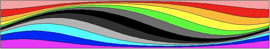
Figure 8: Profile of the
Feedback-CosExp.xml example.
The weighting formula used here adapts an approach described in my 1986 article, “Two Pieces for Amplified Guitar”. What is needed is a formula that favors positions on one side of the circle at the expense of positions on the opposite side. The cosine function, with its peak at 0° and its trough at 180°, has the right shape. However the cosine function goes negative on the back side of the circle, and there's no such thing as a negative weight.
My solution was to use the cosine function as an exponent to a suitable (positive) base. This works because Rcos(x) proceeds from R when x=0°, through 1 when x=90°, through 1/R when x=180°, back through 1 when x=270°, returning to R when x=360°. Thinking about it, we need to replace x with two angles, θ to indicate the position of greatest emphasis and δ to indicate the Chroma position relative to θ. We also need to accomodate the fact that weight contours only accept values in the range from zero to unity. We can do this by dividing Rcos(θ+δ) by its maximum value, R.
Applying this reasoning with R=3 leads us to the formula:
| w(θ,δ) = | 3cos(θ+δ) 3 |
Where
- θ = 2π(t/T)
- t is the current Event start time, expressed in quarter notes.
- T is the total duration of the example, also expressed in quarter notes.
- δ = 2π(k)/12, and
- k is the Chroma index.
With 12 Chromas and 100 Events, 1200 weights need to be calculated to generate the profile shown in Figure 8. Naturally, I didn't input all these weights using the weight contour editor. Instead I created a short Java program to generate the file.
You can witness the selection process for Example #4 by playing the animation above.
In the event that your browser does not support my video formats, I present the composed
result in Figure 9.
Feedback-Evolution.mp3 provides an audio realization of the generated result.
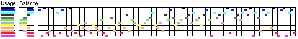
Figure 9: The
Feedback-CosExp.xml example, realized with Heterogenity=0.1 and Seed=0.
Example #5: Diatonic Chords
Example #5 select chords from the D major scale. There are 11 four-note Chords referencing 22 distinct Sounds. The Sounds in turn reference 7 distinct Chromas. As with the previous examples, balance is the ONLY criterion of selection — voice leading is entirely coincidental! The example comprises 100 Events, all of unit duration.
The Chromas detailed in Table 8 correspond to the seven degrees of the D major scale.
| Index | Color | Degree |
| 0 | RED | D |
| 1 | ORANGE | E |
| 2 | YELLOW | F# |
| 3 | GREEN | G |
| 4 | BLUE | A |
| 5 | MAGENTA | B |
| 6 | PINK | C# |
Table 8: Chromas for Example #5.
For this example I chose to define three sets of weights, one set each for the three harmonic functions: tonic, subdominant, and dominant. The tonic degree for D major is D, the subdominant degree is G, and the dominant degree is A. Each of these degrees will be weighted strongly in their corresponding weight sets.
For the other degrees I apply some chord-substitution principles from Michael Rendish of the Berklee College of Music. According to Rendish, in the key of D major:
- Any chord containing F#, but not G, can substitute for the tonic.
- Any chord containing G, but not C#, can substitute for the subdominant.
- Any chord containing G and C# together, but not D, can substitute for the dominant.
Table 9 lists the weights I have selected for each Chroma under tonic, subdominant, and dominant functions. D, G, and A have weight 1.0 in their respective groups, since these degrees are often doubled in the chords enumerated below. Other degrees have weight 0.5 when favored by Rendish's principles, weight 0.0 when Rendish excludes them, and weight 0.3 otherwise.
| Index | Degree | Tonic Weight | Subdominant Weight | Dominant Weight |
| 0 | D | 1.0 | 0.5 | 0.0 |
| 1 | E | 0.3 | 0.3 | 0.3 |
| 2 | F# | 0.5 | 0.3 | 0.3 |
| 3 | G | 0.0 | 1.0 | 0.5 |
| 4 | A | 0.5 | 0.3 | 1.0 |
| 5 | B | 0.3 | 0.3 | 0.3 |
| 6 | C# | 0.3 | 0.0 | 0.5 |
Table 9: Chroma weights for harmonic functions.
Once these three weight sets were defined, I was able to design the profile not as a bundle of weight contours, but rather as a succession of harmonic functions. This resulting profile is detailed in Table 10 and graphed in Figure 10.
| Segment | Time | Duration | Harmony |
| 0 | 0 | 20 | Tonic |
| 1 | 20 | 10 | Tonic to Subdominant |
| 2 | 30 | 10 | Subdominant |
| 3 | 40 | 10 | Subdominant to Tonic |
| 4 | 50 | 10 | Tonic |
| 5 | 60 | 10 | Subdominant |
| 6 | 70 | 10 | Subdominant to Dominant |
| 7 | 80 | 10 | Dominant |
| 8 | 90 | 10 | Tonic |
Table 10: Harmonic profile for
Feedback-Diatonic.xml.
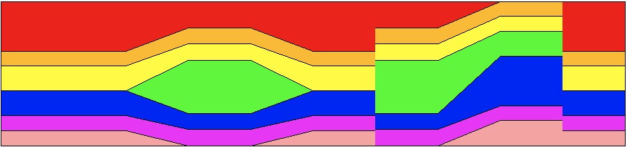
Figure 10: Profile of the
Feedback-Diatonic.xml example.
When you build a feedback scenario in the graphical editor, you need to progress from Chromas to Sounds to Chords. However in conceiving of the thing it is better in some cases to plan from the top down. This is such a case: we need to know what pitches the Chords will use before we can go about defining the Sounds. Table 9 lists the Chords, which all derive from the D major scale.
| Index | Pitch | Pitch | Pitch | Pitch |
| 0 | D2 | F#4 | A4 | D5 |
| 1 | D3 | D4 | F#4 | A4 |
| 2 | D3 | G4 | B4 | G5 |
| 3 | E2 | G3 | B3 | G4 |
| 4 | F#2 | A3 | D4 | A4 |
| 5 | G2 | G4 | B4 | D5 |
| 6 | G3 | D4 | G4 | B4 |
| 7 | A2 | G4 | A4 | C#5 |
| 8 | A3 | C#4 | E4 | G4 |
| 9 | B3 | D4 | F#4 | D5 |
| 10 | C#3 | G4 | A4 | E5 |
Table 11: Chord scheme for Example #5.
I used the Musical Calculator to dedup and sort the pitches in Table 11, obtaining the Sounds listed in Table 12.
| Scale Index | Chroma Index | MIDI Program | MIDI Key | MIDI Velocity |
| 0 | 0 | PIANO_ACOUSTIC_GRAND | D2 | 90 |
| 1 | 1 | PIANO_ACOUSTIC_GRAND | E2 | 90 |
| 2 | 2 | PIANO_ACOUSTIC_GRAND | F#2 | 90 |
| 3 | 3 | PIANO_ACOUSTIC_GRAND | G2 | 90 |
| 4 | 4 | PIANO_ACOUSTIC_GRAND | A2 | 90 |
| 5 | 6 | PIANO_ACOUSTIC_GRAND | C#3 | 90 |
| 6 | 0 | PIANO_ACOUSTIC_GRAND | D3 | 90 |
| 7 | 3 | PIANO_ACOUSTIC_GRAND | G3 | 90 |
| 8 | 4 | PIANO_ACOUSTIC_GRAND | A3 | 90 |
| 9 | 5 | PIANO_ACOUSTIC_GRAND | B3 | 90 |
| 10 | 6 | PIANO_ACOUSTIC_GRAND | C#4 | 90 |
| 11 | 0 | PIANO_ACOUSTIC_GRAND | D4 | 90 |
| 12 | 1 | PIANO_ACOUSTIC_GRAND | E4 | 90 |
| 13 | 2 | PIANO_ACOUSTIC_GRAND | F#4 | 90 |
| 14 | 3 | PIANO_ACOUSTIC_GRAND | G4 | 90 |
| 15 | 4 | PIANO_ACOUSTIC_GRAND | A4 | 90 |
| 16 | 5 | PIANO_ACOUSTIC_GRAND | B4 | 90 |
| 17 | 6 | PIANO_ACOUSTIC_GRAND | C#5 | 90 |
| 18 | 0 | PIANO_ACOUSTIC_GRAND | D5 | 90 |
| 19 | 1 | PIANO_ACOUSTIC_GRAND | E5 | 90 |
| 20 | 3 | PIANO_ACOUSTIC_GRAND | G5 | 90 |
| 21 | 4 | PIANO_ACOUSTIC_GRAND | A5 | 90 |
Table 12: Sounds for
Feedback-Diatonic.xml.
You can witness the selection process for Example #5 by playing the animation above.
In the event that your browser does not support my video formats, I present the composed
result in Figure 11.
Feedback-Evolution.mp3 provides an audio realization of the generated result.

Figure 11: The
Feedback-Diatonic.xml example, realized with Heterogenity=0.1 and Seed=0.
| © Charles Ames | Page created: 2013-09-18 | Last updated: 2017-07-04 |