Discrete Poisson Transform¹

Introduction

The DiscretePoisson transform adapts values from the driver domain to an unbounded integer range, where the weight associated with each range value follows a Poisson distribution.

In Wikipedia's characterization, the Poisson distribution models processes that "count, among other things, the number of discrete occurrences (sometimes called "events" or "arrivals") that take place during a time-interval of given length."

The integers output by DiscretePoisson.convert() are controlled by two parameters implemented as Java fields. Field mean (symbolized λ) is a double-precision number corresponding to the average waiting time between occurrences. Field extent establishes a practical upper limit upon the nominally unbounded output range. This limit is measured in standard deviations. The examples which follow fix extent at 6.

The point density function f(k) is:

f(k) =

λ^ke^−λ

Where the symbol e represents Euler's number and the exclamation point indicates factorial. Wikipedia attributes this formula to French mathematician Siméon Denis Poisson The Poisson distribution is an essential component of the Poisson point process, which Wikipedia indicates that Poisson the mathematician never studied. This seems inconsistent to me given the intimate relationship between the discrete Poisson distribution and the continous exponential distribution described here.

For the Poisson family of point density functions, the parametric mean (average, symbolized μ) is λ while the parametric variance (squared deviation, symbolized σ²) is also λ. The range of the Poisson distribution is bounded by zero on the left and unbounded to the right. Point densities tail out to zero as range values increase. As λ increases beyond unity, the point density at zero drops away, and a hump develops around λ.

Profile

The two panels presented as Figure 1 (a) and Figure 1 (b) illustrate the influence which DiscretePoisson.convert() exerts over driver sequences. The horizontal k axis shows the sample values v_k which have been obtained from driver values x_k using convert(). Each left-side sample graph presents 200 values; the right-side histogram presents a sidewise bar for each range value.

The source sequences used to create Figure 1 (a) and Figure 1 (b) are the same sequences used to create the profile panel for ContinuousUniform, which passes through its driver values undecorated. You can view the actual source sequences by clicking the link. All three source sequences are nominally uniform. The first source is standard randomness from Lehmer. The second source is balanced-bit values from Balance. The third source is an ascending succession produced using DriverSequence.

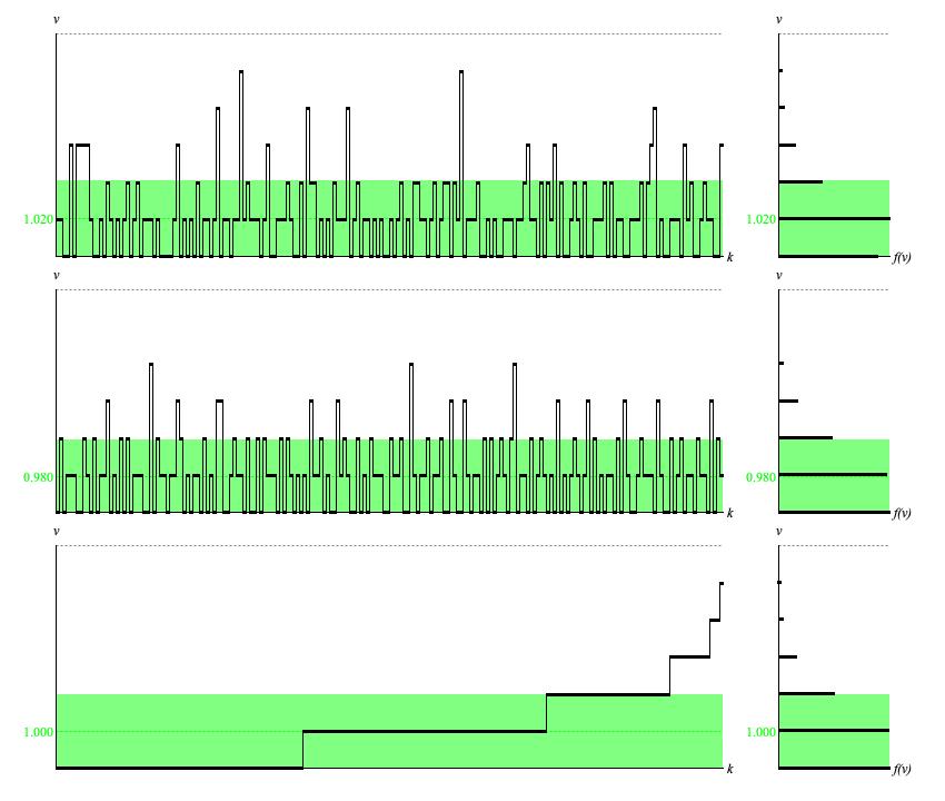
Figure 1 (a): Panel of DiscretePoisson output when mean=1. Each row of graphs provides a time-series graph of samples (left) and a histogram analyzed from the same samples (right). The first row of graphs was generated using the standard random number generator. The second row was generated using the balanced-bit generator. The third row was generated using an ascending sequence of driver values, equally spaced from zero to unity.

The vertical v axis in Figure 1 (a) ranges from 0 to 6; that is, the application range from 0 to 5 and the number of outcomes, 6.

For Figure 1 (a) the parametric mean is

μ = λ = 1.000.

The parametric deviation is:

σ = √λ = √1 = 1.000.

The standard-random time-series (top row of Figure 1 (b)) bears comparison to the corresponding top-row graphic for DiscreteUniform, which employed the same random source sequence. The relative ups and downs are much alike. The calculated average of 1.020 differs from μ = 1.000 by 2%. The calculated deviation of 1.044 around this average differs from σ = 1.000 by 4%. However the top-row histogram differs noticably from the bottom-row histogram, which presents ideal point densities.

The balanced-bit time-series (middle row of Figure 1 (a)) likewise bears comparison to the corresponding middle-row graphic for DiscreteUniform, which employed the same balanced-bit source sequence. Again, the relative ups and downs are much alike. The calculated average of 0.980 differs from μ = 1.000 by 2%. The calculated deviation of 0.974 around this average differs from σ = 1.000 by 2.5%. The middle-row histogram is barely distinguishable from the bottom-row histogram.

The time-series graph generated using ascending, equally spaced driver values (bottom row of Figure 1 (a)) presents the quantile function for the Poisson distribution with the indicated mean. This is an irregular ascending step function, where the run of each step indicates the point density and the rise is fixed at one unit. The bottom-row histogram of sample values presents the distribution's probability density function or PDF.

The numerical average of 1.000 is indistinguishable from μ = 1.000. by 3%. The numerical standard deviation of 1.005 around this average differs from σ = 1.000 by 0.5%. I reran this graph raising extent=5 to 16 and got the same discrepancy.

The 1.000−1.005 is less than zero, so the light-green shaded interval ranges from 0.00 to 1.000+1.005 = 2.005. The light-green band is therefore 2.005/5 = 0.37 = 37% of the full application range from 0 to 5. Since the continuous uniform distribution had 58% of samples within ± one standard deviation of the mean, this suggests that with the Poisson transform with mean = 1 is squeezing 58% of samples into 37% of the application range, giving a concentration rate of 58/37 = 1.57.

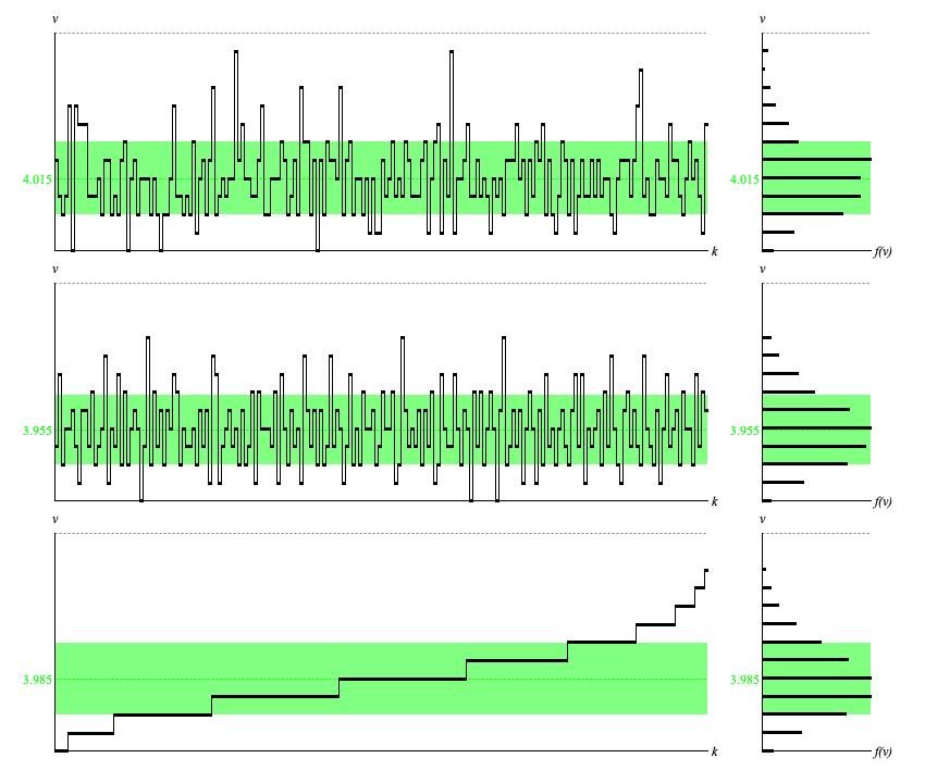
Figure 1 (b): Panel of DiscretePoisson output when mean=4. Each row of graphs provides a time-series graph of samples (left) and a histogram analyzed from the same samples (right). The first row of graphs was generated using the standard random number generator. The second row was generated using the balanced-bit generator. The third row was generated using an ascending sequence of driver values, equally spaced from zero to unity.

The vertical v axis in Figure 1 (a) ranges from 0 to 12; that is, the application range from 0 to 11 and the number of outcomes, 12.

For Figure 1 (a) the parametric mean is

μ = λ = 4.000.

The parametric deviation is:

σ = √λ = √4 = 2.000.

The standard-random time-series (top row of Figure 1 (b)) bears comparison to the corresponding top-row graphic when λ = 1. The relative ups and downs are the same. The calculated average of 4.015 differs from μ = 4.000 by 0.8%. The calculated deviation of 2.014 around this average differs from σ2.000 by 0.7%. However the top-row histogram differs noticably from the bottom-row histogram, which presents ideal point densities.

The standard-random time-series (top row of Figure 1 (b)) bears comparison to the corresponding middle-row graphic when N = 1. The relative ups and downs are the same. The calculated average of 3.955 differs from μ = 4.000 by 1%. The calculated deviation of 1.924 around this average differs from σ = = 2.000 by 4%. The middle-row histogram is barely distinguishable from the bottom-row histogram.

The time-series graph generated using ascending, equally spaced driver values (bottom row of Figure 1 (b)) presents the quantile function for the poisson distribution with the indicated parameters. This is an irregular ascending step function, where the run of each step indicates the point density and the rise is fixed at one unit. The bottom-row histogram of sample values presents the distribution's probability density function or PDF.

The numerical average of 3.985/span> differs from μ = 4.000 by 0.4%. Increasing extent to 7 brings the numerical average up to 3.995 while also extending the vertical range of the graph up to 13. Larger extents brought no further improvement. The numerical standard deviation of 1.974 around this average differs from σ = 2.000 by 2.5%.

The interval from 3.985−1.974 = 2.011 to 3.985+1.974 = 5.959 is 2*1.974/11 = 0.358 = 36% of the full application range from 0 to 11. Since the continuous uniform distribution had 58% of samples within ± one standard deviation of the mean, this suggests that with the Poisson transform with mean = 4 is squeezing 58% of samples into 36% of the application range, giving a concentration rate of 58/37 = 1.61.

/**
 * The {@link DiscretePoisson} class implements a discrete statistical
 * transform based on the Poisson distribution. This distribution models
 * rare events such as cars passing by on a road (but not during rush hour),
 * or such as beta emissions from a radioactive substance.
 * There are, in fact, two Poisson distributions.  One models the durations
 * spent waiting between rare events; this is known known as the negative
 * exponential distribution and it is discussed as a limiting case for the
 * {@link ContinuousMyhill} transform.  The distribution officially named for
 * Poisson models how many rare events occur during an interval of time.
 * The one parameter controlling the Poisson distribution is the average
 * event density &lambda;. The {@link #mean} field of the {@link DiscretePoisson}
 * class stands in for the average event density &lambda;.
 * As a statistical transform, {@link DiscretePoisson} does not itself employ
 * probability or randomness. Instead it responds to an externally generated
 * driver sequence which may or may not be random.
 * {@link DiscreteDistribution#quantile(double)} converts the driver value
 * to an outcome.
 * @author Charles Ames
 */
public class DiscretePoisson extends DiscreteDistributionTransform {
   /**
    * Determines average number of events per time unit.
    */
   private double mean;
   /**
    * Determines the range extent in standard deviations.
    */
   private double extent;
   /**
    * Constructor for {@link DiscretePoisson} instances.
    * @param container An entity which contains this transform.
    */
   public DiscretePoisson(WriteableEntity container) {
      super(container);
      this.mean = Double.NaN;
      this.extent = Double.NaN;
   }
   /**
    * Getter for {@link #mean} .
    * @return The assigned {@link #mean} value.
    * @throws UninitializedException when {@link #mean} has not
    * been initialized.
    */
   public double getMean() {
      if (Double.isNaN(mean))
         throw new UninitializedException("Mean not initialized");
      return mean;
   }
   /**
    * Setter for {@link #mean}.
    * @param mean The intended {@link #mean} value.
    * @return True if {@link #mean} has changed; false otherwise.
    */
   public boolean setMean(double mean) {
      checkMean(mean);
      if (this.mean != mean) {
         this.mean = mean;
         invalidate();
         makeDirty();
         return true;
      }
      return false;
   }
   /**
    * Check if the indicated value is suitable for {@link #mean}.
    * @param mean The indicated value.
    */
   public void checkMean(double mean) {
      if (MathMethods.TINY > mean)
         throw new IllegalArgumentException("Mean not positive");
   }
   /**
    * Setter for {@link #extent}.
    * @param extent The intended {@link #extent} value.
    * @return True if {@link #extent} has changed; false otherwise.
    */
   public boolean setExtent(double extent) {
      checkExtent(extent);
      if (this.extent != extent) {
         this.extent = extent;
         invalidate();
         makeDirty();
         return true;
      }
      return false;
   }
   /**
    * Getter for {@link #extent} .
    * @return The assigned {@link #extent} value.
    * @throws UninitializedException when {@link #extent} has
    * not been initialized.
    */
   public double getExtent() {
      if (Double.isNaN(extent))
         throw new UninitializedException("Extent not initialized");
      return extent;
   }
   /**
    * Check if the indicated value is suitable for {@link #extent}.
    * @param extent The indicated value.
    */
   public void checkExtent(double extent) {
      if (2. > extent)
         throw new IllegalArgumentException(
            "Extent must exceed two standard deviations");
   }
   @Override
   protected void validate(DistributionBase<Integer> distribution) {
      ((DiscreteDistribution) distribution).calculatePoisson(
         getMean(), getExtent());
   }
}

Listing 1: The DiscretePoisson implementation class.

Coding

The type hierarchy for DiscretePoisson is:

TransformBase<T extends Number> extends WriteableEntity implements Transform<T>
DiscreteDistributionTransform extends TransformBase<Integer> implements Transform.Discrete
DiscretePoisson extends DiscreteDistributionTransform

DiscreteDistributionTransform embeds a DiscreteDistribution which manages the succession of value-weight items.

Each DiscretePoisson instance internally maintains a DiscreteDistribution instance whose succession of items is populated by the call to DiscreteDistribution.calculatePoisson() in method DiscretePoisson.validate(). This call to calculatePoisson() creates lambda*extent items with weights according to the point density function given above.

The distributing step of conversion happens in DiscreteDistributionTransform, where the convert() method does this:

return getDistribution().quantile(driver);

TransformBase maintains a valid field to flag parameter changes. This field starts out false and reverts to false with every time DiscretePoisson calls TransformBase.invalidate(). This happens with any change to mean or extent. Any call to TransformBase.getDistribution() (and DiscreteDistributionTransform.convert() makes such a call) first creates the distribution if it does not already exist, then checks valid. If false, then getDistribution() calls validate(), which is abstract to TransformBase but whose implementation is made concrete by DiscretePoisson. And that particular implementation of validate() makes use of DiscreteDistribution.calculatePoisson(getMean()), getExtent()) to recalculate the distribution items.

Comments

The present text is adapted from my Leonardo Music Journal article from 1991, "A Catalog of Statistical Distributions". The heading is "Poisson", p. 60.

Page created: 2022-08-29

Last updated: 2022-08-29

Discrete Poisson Transform1

Introduction

Profile

Coding

Comments

Discrete Poisson Transform¹