Discrete Negative Binomial Transform1
Introduction
The DiscreteNegativeBinomial transform adapts
values from the driver domain to an unbounded integer range, where the weight associated with
each range value follows a negative binomial distribution,
which is attributed to Blaise Pascal.
The negative binomial distribution enriches Jakob Bernoulli's urn model. The scenario involves an open-ended succession of Bernoulli trials. These trials are independent; that is, the outcome of one trial has no influence upon any other trial, and they are identically distributed, which means that all trials have the same probability p of success. The scenario counts the number k of successful trials until N failures have occurred.
The integers output by DiscreteNegativeBinomial.convert() are
controlled by three parameters implemented as Java fields. Field failures
is an integer corresponding to the allowed number of failures N in the urn scenario.
Field weight is a double-precision number corresponding to the probability of
single-trial success p in the urn scenario. This second field ranges from zero (always fails) to
unity (always succeeds). Field extent establishes a practical upper limit
upon the nominally unbounded output range. This limit is measured in standard deviations. The examples which follow fix
extent at 5.
The point density function f(k) is:
| f(k) = |
|
pk(1−p)N |
Where the exclamation point indicates factorial. Wikipedia says otherwise about the point density function.2
For the negative binomial family of point density functions, the parametric mean (average, symbolized μ) is given by some sources (including Wikipedia) as Np/(1−p) while the parametric variance (squared deviation, symbolized σ2) is given as Np/(1−p)2.
The graph of the negative binomial distribution starts out with a hump and tails out to zero as values increase. As p grows toward unity, the number of trials expodes while the distinction between consecutive values melts away. The negative binomial distribution thus converges to a gamma distribution, a continuous curve which is also left-bounded at zero, which also starts with a hump, and which also tails out to zero on the right. This gamma distribution has shape parameter N and scale parameter p/(1−p).3
The negative binomial distribution with N=1 is called a geometric distribution. As p grows toward unity, a geometric distribution converges to an exponential distribution (also called "negative exponential") with mean p/(1−p). Geometric is to negative binomial as exponential is to gamma.
Profile
The two panels presented as Figure 1 (a) and Figure 1 (b) illustrate the influence which
DiscreteNegativeBinomial.convert() exerts over driver sequences.
The horizontal
k axis shows the sample values vk which have been obtained
from driver values xk using
convert(). Each left-side sample graph presents 200 values; the right-side
histogram presents a sidewise bar for each range value.
The source sequences used to create Figure 1 (a) and Figure 1 (b) are the same
sequences used to create the profile panel for ContinuousUniform,
which passes through its driver values undecorated. You can view the actual
source sequences by clicking the link. All three source sequences are nominally uniform.
The first source is standard randomness from Lehmer.
The second source is balanced-bit values from Balance.
The third source is an ascending succession produced using DriverSequence.

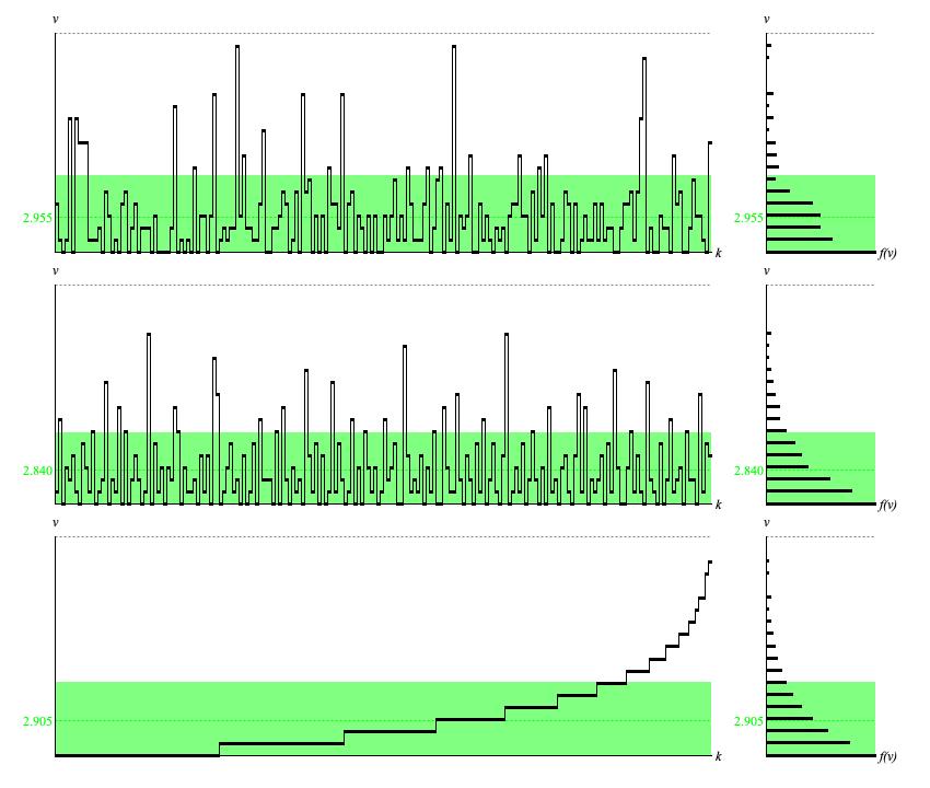
Figure 1 (a): Panel of
DiscreteNegativeBinomial output
when failures=1 and weight=0.7.
Each row of graphs provides a time-series graph of samples (left)
and a histogram analyzed from the same samples (right).
The first row of graphs was generated using the standard random number generator. The second
row was generated using the balanced-bit generator. The third row was generated using an ascending sequence of driver values,
equally spaced from zero to unity.
Having failures=1, Figure 1 (a) conforms to a
geometric distribution.
The vertical v axis in Figure 1 (a) ranges from 0 to 18; that is, the application range
from 0 to 17 and the number of outcomes, 18.
For Figure 1 (a) the parametric mean is
The parametric deviation is:
The standard-random time-series (top row of Figure 1 (b)) bears comparison to the corresponding
top-row graphic for DiscreteUniform,
which employed the same random source sequence. The relative ups and downs are much alike.
The calculated average of 2.955 differs from μ = 3.000
by 1.5%.
The calculated deviation of 3.377 around this average differs from σ = 3.462
by 2.4%. However the top-row histogram differs noticably from the bottom-row histogram, which
presents ideal point densities.
The balanced-bit time-series (middle row of Figure 1 (a)) likewise bears comparison to the corresponding
middle-row graphic for DiscreteUniform,
which employed the same balanced-bit source sequence. Again, the relative ups and downs are much alike.
The calculated average of 2.840 differs from μ = 3.000
by 5%.
The calculated deviation of 3.055 around this average differs from σ = 3.462
by 12%. The middle-row histogram is barely distinguishable from the bottom-row histogram.
The time-series graph generated using ascending, equally spaced driver values (bottom row of Figure 1 (a)) presents the quantile function for the bernoulli distribution with the indicated parameters. This is an irregular ascending step function, where the run of each step indicates the point density and the rise is fixed at one unit. The bottom-row histogram of sample values presents the distribution's probability density function or PDF.
The numerical average of 2.905 differs from μ = 3.00
by 3%. This discrepancy happens because extent=5.
Bringing the numerical average up to 2.99 requires increasing extent to
16; however, this would extend the vertical range of the graph up to 55, with few or none of the additional options ever being selected.
The numerical standard deviation of 3.181 around this average differs from σ = 3.462
by 8%. Increasing extent to 16 gives a standard deviation of
3.484 and reduces the discrepancy to 0.6%.
The 2.905−3.181 is less than zero, so the light-green shaded interval ranges from 0.00 to
2.905+3.181 = 6.37. Since 6.37/17 = 0.37 = 37% of the full application range
from 0 to 17. Since the continuous uniform distribution
had 58% of samples within ± one standard deviation of the mean, this suggests that with the negative binomial transform
with failures = 1 and weight = 0.75
is squeezing 58% of samples into 37% of the application range, giving a concentration rate of 58/37 = 1.57.

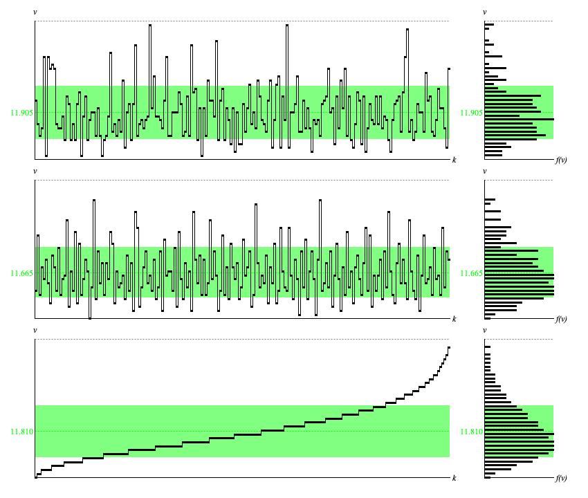
Figure 1 (b): Panel of
DiscreteNegativeBinomial output
when failures=4 and weight=0.7.
Each row of graphs provides a time-series graph of samples (left)
and a histogram analyzed from the same samples (right).
The first row of graphs was generated using the standard random number generator. The second
row was generated using the balanced-bit generator. The third row was generated using an ascending sequence of driver values,
equally spaced from zero to unity.
The vertical v axis in Figure 1 (a) ranges from 0 to 38; that is, the application range from 0 to 37 and the number of outcomes, 38.
For Figure 1 (b) the parametric mean is
The parametric deviation is:
The standard-random time-series (top row of Figure 1 (b)) bears comparison to the corresponding top-row graphic when N = 1. The relative ups and downs are the same. The calculated average of 11.905 differs from μ = 12.000 by 0.8%. The calculated deviation of 6.659 around this average differs from σ6.928 by 4%. However the top-row histogram differs noticably from the bottom-row histogram, which presents ideal point densities.
The standard-random time-series (top row of Figure 1 (b)) bears comparison to the corresponding middle-row graphic when N = 1. The relative ups and downs are the same. The calculated average of 11.665 differs from μ = 12.000 by 2.8%. The calculated deviation of 6.378 around this average differs from σ = = 6.928 by 8%. The middle-row histogram is barely distinguishable from the bottom-row histogram.
The time-series graph generated using ascending, equally spaced driver values (bottom row of Figure 1 (b)) presents the quantile function for the negative binomial distribution with the indicated parameters. This is an irregular ascending step function, where the run of each step indicates the point density and the rise is fixed at one unit. The bottom-row histogram of sample values presents the distribution's probability density function or PDF.
The numerical average of 11.810 differs from μ = 12.000
by 3%. This discrepancy happens because extent=5.
Increasing extent to 16 brings the numerical average up to 11.975 while also
extending the vertical range of the graph up to 110.
The numerical standard deviation of 6.564 around this average differs from σ = 6.928
by 8%. Increasing extent to gives a standard deviation of
6.860 and reduces the discrepancy to 0.6%.
The interval from 11.810−6.564 = 5.246 to 11.810+6.564 = 18.374 is
2*6.564/37 = 0.355 = 36% of the full application range from 0 to 37. Since the continuous uniform distribution
had 58% of samples within ± one standard deviation of the mean, this suggests that the negative binomial transform
with failures = 4 and weight = 0.75
is squeezing 58% of samples into 37% of the application range, giving a concentration rate of 58/37 = 1.57.
DiscreteNegativeBinomial implementation class.
Coding
The type hierarchy for DiscreteNegativeBinomial is:
-
TransformBase<T extends Number> extends WriteableEntity implements Transform<T> -
DiscreteDistributionTransform extends TransformBase<Integer> implements Transform.Discrete -
DiscreteNegativeBinomial
                  extends DiscreteDistributionTransform
DiscreteDistributionTransform
embeds a DiscreteDistribution
which manages the succession of value-weight items.
Each DiscreteNegativeBinomial instance internally maintains a
DiscreteDistribution instance
whose succession of items is populated by the call to
DiscreteDistribution.calculateNegativeBinomial()
in method DiscreteNegativeBinomial.validate().
This call to calculateNegativeBinomial() creates
σ×extent items
with weights according to the point density function given above.
The distributing step of conversion happens in DiscreteDistributionTransform,
where the convert() method does this:
return getDistribution().quantile(driver);
TransformBase maintains a valid field
to flag parameter changes. This field starts out false
and reverts to false with every time DiscreteNegativeBinomial
calls TransformBase.invalidate(). This happens
with any change to failures, weight,
or extent. Any call to
TransformBase.getDistribution()
(and DiscreteDistributionTransform.convert() makes such a call)
first creates the distribution if it does not already exist, then checks valid. If
false, then getDistribution() calls
validate(), which is abstract to
TransformBase but whose implementation is
made concrete by DiscreteNegativeBinomial. And that particular implementation of
validate()
makes use of DiscreteDistribution.calculateNegativeBinomial(getFailures(), getWeight()), getExtent()) to recalculate the
distribution items.
Comments
- The present text is adapted from my Leonardo Music Journal article from 1991, "A Catalog of Statistical Distributions". The heading is "Negative Binomial", p. 60.
- The formula given by Wikipedia reverses the exponents for p and (1−p). However the value raised to exponent k controls the rate of tail-off, Higher values of p means greater trial success rates, which means that tails should spread out as p increases.
-
An online paper by Tim Barry,
"Gamma, Poisson, and negative binomial distributions"
(June 16, 2020) gives the point-density function which I actually use in
DiscreteDistribution.calculateNegativeBinomial(). This paper is also my source for the value p/(1−p) given for the gamma distribution's scale parameter.
| © Charles Ames | Page created: 2022-08-29 | Last updated: 2022-08-29 |