Linearity
Introduction
A signal-processing algorithm is said to be linear if its graph conforms to a straight line. The characterization is important because non-linear algorithms cause signal distortion, while linear algorithms don't.
Geometry tells us that a line is the shortest path between two points. More informatively, analytical geometry tells us that a line is a mathematical function whose slope is everywhere constant. Now analytic geometry has x and y axes (which classical geometry doesn't), and one cannot say that slope is rise/run without knowing that run is a displacement along the x axis and that rise is a displacement along the y axis.
The topic of this page is linearity, but getting there requires some supporting concepts. First off is the idea of a mathematical function. This idea, the function, is the category of which the line graph is a member. Knowing functions, we then need to understand how line graphs are distinguished from other functions. That attribute is constancy of slope. So second off is the idea of slope, what it means, how to use function values to calculate slope even when it is not constant, and what slope does to reshape signals as they are processed through algorithms.
Mathematical Functions
Understanding mathematical functions in general is necessary because signal-processing algorithms typically use functions to transform signals, and linear functions are just one available option.
The notion of a function was first introduced into mathematics by Gottfried Leibniz and used by him to explain his invention, the calculus.1 A function may be described as a rule of association between elements of two sets:
- The domain described by one or more "independent" variables, and
- the range described by one "dependent" variable.
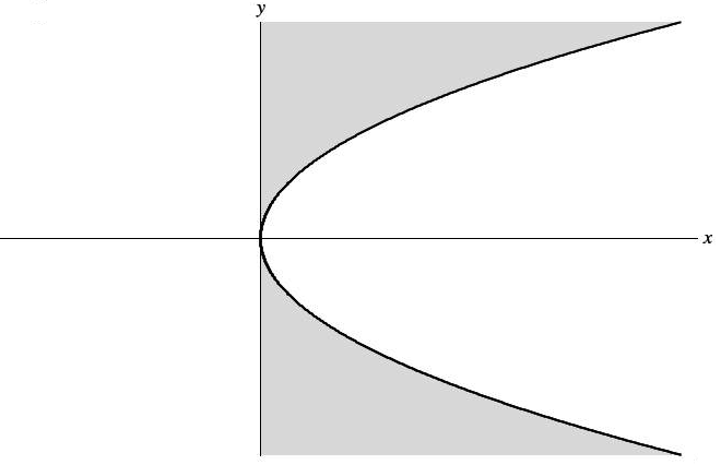
The rule of association is subject to a restriction: any single point or coordinate in the domain may never map to more than one value in the range. One formula which does not conform to this restriction is the formula y2 = x graphed in Figure 1. The graph shows a parabola tipped on its side. The formula is undefined for negative x values, has one y value when x = 0 and two y values when x is positive.
Solving for y gives:
Convention states that the radical (√) extracts the positive square root of its content; hence the ± sign is required to indicate that y could be either +√x or −√x. Since no single value of x may map to more than one y, the formula y2 = x does not qualify as a function.
Discarding that portion of the graph which lies beneath the x axis produces the formula:
This modified formula does qualify as function whose domain and range are both sets of non-negative real numbers. However the slope of √x is not everywhere constant; rather it starts out nearly vertical when x is just slightly vertical and it continually moderates in steepness as x increases. Thus y = √x cannot be a linear function.
Euler, who inherited the function concept through studies with Leibnitz's friend Bernoulli, introduced the notation f(x) to indicate that the value of function f depends upon the value of the (independent) variable x. When the domain has just the one independent variable x, then f(x) describes a never-vertical curve. When the domain has two independent variables x and y, then f(x,y) describes a surface.
There are additional restrictions which we need to impose; these restrictions come about because our ultimate purpose is to process audio signals. The functions we're considering here should never introduce pops or clicks. If you are at all familiar with audio signal processing, then you know that a nasty click will result when a signal is discontinuous; that is when it jumps abruptly between two separated values. However you may not also know that pops and clicks also happen where a signal has a kink;2 for example, when a rising function abruptly turns downward. Now when a signal processes through a function which is discontinuous or kinky, then the function will impress its discontinuities and kinks onto its output. Thus the functions we're considering here must be nowhere discontinuous and nowhere kinky.
Slopes
Stipulate that the function f proceeds smoothly, with neither discontinuities nor kinks. We now drill down into the behavior f over the interval from x1 to x2. The distance from x1 to x2 is called the run of f during the interval. If the run is short enough, then the behavior of f can be approximated by a chord (straight line) running diagonally from (x1,f(x1)) to (x2,f(x2)). The distance from f(x1) to f(x2) is called the rise of f during the interval.
The slope of function f during the interval from x1 to x2 calculates the ratio of rise to run:
|
= |
|
Ascending Slope
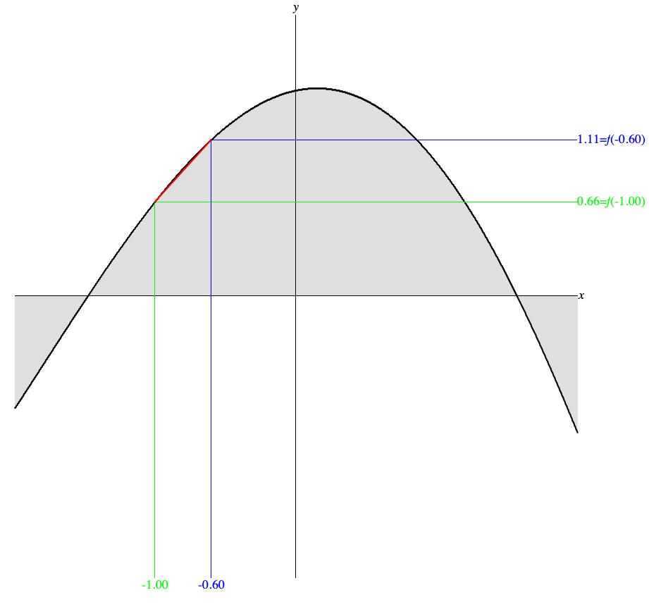
Figure 2 (a) applies this formula to function f, plotted as a thick black curve with a local maximum somewhat to the right of the y axis. In particular, Figure 2 (a) illustrates how the slope behaves over an interval during which the function f ascends. The vertical green line segment indicates the lower limit of the interval at x1 = -1.00 while the vertical blue line segment indicates the upper limit of the interval at x2 = -0.60.
Notice the horizontal green line segment whose left begins where the segment for x1 = -1.00 intersects function f. The corner formed between these two green segments, vertical and horizontal, graphically locates f(-1.00) (the value of f when x1 = -1.00) at 0.66.
Likewise notice the horizontal blue line segment whose left begins where the segment for x2 = -0.60 intersects function f. The corner formed between these two blue segments graphically locates f(-0.60) (the value of f when x2 = -0.60) at 1.11.
Thus over the interval from x1 = -1.00 to x2 = -0.60, the run is:
while the rise is:
and the slope is:
| = |
|
= |
|
= 1.125 |
One remaining graphic component of Figure 2 (a) still requires explanation. This is the red line segment (or chord) from (x1,f(x1)) = (-1.00,1.11) to (x2,f(x2)) = (-0.60,0.66). The slope of 1.125, is strongly positive; hence the chord angles upward to the right. As suggested previously, this line segment approximates the behavior of f(x) as x proceeds from x1 to x2. The accuracy of this approximation is attested by how the black curve barely peeks out from underneath the red segment.
Descending Slope
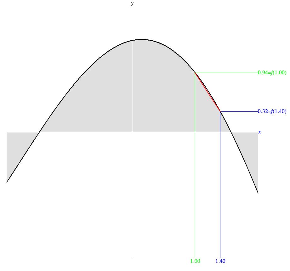
Figure 2 (b) illustrates what happens when the slope is calculated over an interval during which function f descends. The vertical green line segment in Figure 2 (b) indicates the lower limit of the interval at x1 = 1.00 while the vertical blue line segment indicates the upper limit of the interval at x2 = 1.40.
The horizontal green line segment whose left begins where the segment for x1 = 1.00 intersects function f graphically locates f(1.00) at 0.94. The horizontal blue line segment whose left begins where the segment for x2 = 1.40 intersects function f graphically locates f(1.40) at 0.32.
The slope from x1 = 1.00 to x2 = 1.40 is:
| = |
|
= |
|
= |
|
= -1.55 |
Figure 2 (b) also contains a red chord (line segment) from (x1,f(x1)) = (1.00,0.94) to (x2,f(x2)) = (1.40,0.32). The slope of -1.55, is strongly positive; hence the chord angles downward to the right. The approximation to f(x) is still good even though a sliver of gray peeks out between the black curve and the red chord.
Nearly Flat Slope
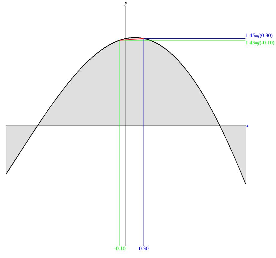
Figure 2 (c) illustrates what happens when the slope is calculated over an interval during which function f crests at a local maximum. The vertical green line segment in Figure 2 (c) indicates the lower limit of the interval at x1 = -0.10 while the vertical blue line segment indicates the upper limit of the interval at x2 = 0.30.
The horizontal green line segment whose left begins where the segment for x1 = -0.10 intersects function f graphically locates f(-0.10) at 1.43. The horizontal blue line segment whose left begins where the segment for x2 = 0.30 intersects function f graphically locates f(0.30) at 1.45.
The slope from x1 = -0.10 to x2 = 0.30 is:
| = |
|
= |
|
= |
|
= 0.05 |
The approximating chord in Figure 2 (c) slopes slightly upward from (x1,f(x1)) = (-0.10,1.43) to (x2,f(x2)) = (0.30,1.45). The slope of 0.05, is only just positive; hence the chord is very near to horizontal. This is the least accurate approximation of f so far, and the explanation is the pronounced curvature of f as the function transitions through its local maximum.
Slope in the Real World
In the physical world, going up consumes energy and going down releases energy. To enrich one's intuitive grasp of slope, it is helpful to consider slope's physical manifestations. Keep in mind however that this page is ultimately concerned with signal processing and that signal processing is uninfluenced by gravity. So regard the present topic as enrichment. Considerations more relevant to signal processing will be explored in the topic following, on Slope and Density.

Structures like roads and waterways can all be regarded as inclined planes with gravity contributing downward acceleration. Structural engineers, who design such things, refer to slope as grade, which quantity engineers always express as a percentage. As Steven Holzner of dummies.com explains, an inclined plane splits gravitational acceleration into the two components shown graphically in Figure 3. In Figure 3, θ indicates the angle of inclination, while the gray box represents a load positioned on the plane.
One component is directed perpendicular to the plane with magnitude g×cos(θ). This perpendicular component acts through the agency of friction to fix the load in place.
The second component is directed parallel to the plane with magnitude g×sin(θ). This parallel component determines the propensity for sideways slippage. Holzner explains why the θ which Figure 3 indicates in red matches the angle of inclination. This means that sin(θ) is obtained by dividing the triangle's rise (the length of the vertical edge at the left) by the triangle's hypontenuse. But for θ ≤ 12 the triangle's run is near enough in length to the triangle's hypontenuse that sin(θ) comes within one percentage point of the slope.
| Category | Grade | θ |
|---|---|---|
| Parking | 5% | 3° |
| Firetruck | 8% | 5° |
| Public Road | 12% | 7° |
| Driveway | 15% to 21% | 9° to 12° |
Table 1: Local bylaws for icy road conditions (after "whistler" at archinect.com/forum).
Table 1 lists maximum grades for icy (low friction) conditions according to "local bylaws" known to its author. Ice mitigates the fixing effect of the perpendicular force. I presume that the 5% entry for the bylaw labeled "Parking" is there to protect parked vehicles from sliding into one another. This would be consistent with advice offered by Eric Sorensen at ayresassociates.com:
Generally a rural roadway cross slope — such as a banked curve — is desired to be no more than 4% [2°] to minimize the chance that a car that is traveling slowly or waiting to turn left onto an intersecting road would slide sideways down the cross slope and into oncoming traffic.
Anyone familar with the adventure of driving around San Francisco (especially with a stick shift) should be glad that city does not experience icy conditions such as those we suffer in the Northeast. According to 7x7.com, the most notorious street grades in San Francisco range upward from 31% (18°). The worst of these grades is "Bradford above Tompkins", at 41% (24°).
Turning from cars and trucks to trains. In theory trains move freight more efficiently because of how the rails reduce the tractive effort required to shift a heavy load. According to RepublicLocomotive.com, tractive effort T in pounds relates to horsepower P and speed S in mph by the formula T = 375P/S. Thus a locomotive exerting 4000 horsepower to pull a train at 30 mph could exert a tractive effort of 375×4000/30 = 50000 pounds. Since 5 pounds per ton of train weight is required to move on straight level track, and since according to Model Railroader Magazine a filled hopper car can weigh some 130 tons, 50000 pounds of tractive effort is enough to pull 50000/5=10000 tons, or 76 hopper cars. However, each percent of grade requires 20 pounds of tractive effort per ton of train weight. A 1% grade drops this capability to 50000/25=2000 tons, or 15 hopper cars. For a 1.5% grade (0.859°), the maximum recommended in 1970 by the U.S. Army for military purposes, the capability would be 50000/35=1428, or 10 hopper cars. For a 2% grade (1.146°), allowed for short runs under exceptional conditions, the capability would be 50000/45=1111, or just 8 hopper cars.
The design of aqueducts requires a grade that is just steep enough to encourage water to flow, but shallow enough to evade erosion damage. According to Wikipedia, the treatise De architectura by Vitruvius (1st centry BC) recommends a gradient of not less than 1 in 4800 (0.021% or 0.012°) to prevent water from pooling. Wikipedia reports that "This value agrees well with the measured gradients of surviving masonry aqueducts." Some Roman aqueduct grades descend as steeply as 1 in 700 (0.143% or 0.082°).
The slope for canals should be 0, since the point of a canal is simply to float the barge, whose motive force is provided by a mule. From Hydrology and Environmental Aspects of Erie Canal (1817-99), 1976.
To save lockage, the [1811] Commissioners took the greatest slope they considered wise, and in a canal 4 feet deep, at a grade of 6 inches per mile, the velocity would be about 1.5 feet per second (1.0 mph) somewhat large for a horse-drawn barge.
A grade of 6 inches per mile resolves to 0.019% (0.011°) — short of the minimum recommended by Vitruvius, but then again, pooling is desirable for a canal. However a later commission opted to eliminate even that miniscule grade and go for a "fully locked" design.
Slope and Density
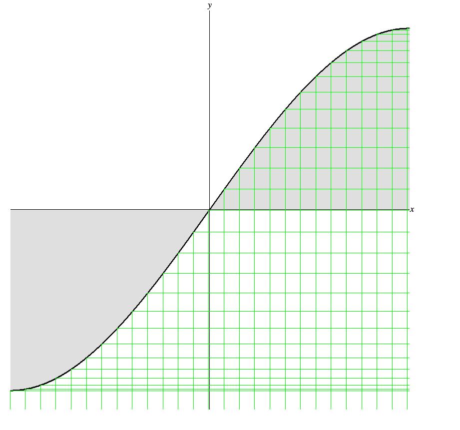
Another way to appreciate the slope is to consider how it effects the density of values as they map from the domain to the range. In Figure 4 illustrates what happens when an independent sequence of evenly spaced x values is plotted against the dependent sequence of corresponding f(x) values. For simplicity's sake the function f is strictly monotonic, which is mathspeak for ever-increasing. Having an always-positive slope eliminates the complication of f(x) values folding back upon themselves. Also for simplicity's sake f is an odd function, meaning f(-x) = -f(x).
Let xn be one particular member of the x sequence, with successor xn+1. Then we can graphically derive the slope near xn by constructing a right triangle whose base (the run) extends from (xn,f(xn)) to (xn+1,f(xn)), whose vertical leg (the rise) extends from (xn+1,f(xn)) to (xn+1,f(xn+1)), and whose hypotenuse extends from (xn,f(xn)) to (xn+1,f(xn+1)).
Despite being continuous and kink-free, despite being monotonic and odd, function f is decidedly nonlinear. Slopes are steep near the y axis and gradual near the left and right edges. The function's impact upon how f(x) values are spaced follows directly from the slope where x is:
- When xn is near to the y axis (near to zero), the vertical leg of the triangle is taller than the base is wide. Rise exceeds run, therefore the slope exceeds unity. The action of f is to space f(x) values more widely than the corresponding x values. Changes in x are amplified.
- When xn is near either to the left edge or to the right edge, the vertical leg of the triangle is shorter than the base is wide. Rise falls short of run, therefore the slope falls short of unity. The action of f is to space f(x) values more narrowly than the corresponding x values. Changes in x are attenuated.
- When xn is either midway between to the left edge and the y axis or midway between to the y axis and the left edge, the vertical leg of the triangle is comparable in length to the base. Rise matches run, tending the slope toward unity. The action of f is to space f(x) values similarly than the corresponding x values. Changes in x are simply passed along.
Linear Functions
The term "linear" comes from geometry, where it identifies the simplest kind of graph, i.e., a straight line. Straight lines have two essential features: they are continuous, and their slope is everywhere constant. (The first feature actually follows from the second.)
Geometry also teaches that two points determine a line. Suppose that the function f is linear. Having two points at (x1,f(x1)) (x2,f(x2)) certainly allows one to calculate the slope of f over the interval from x1 to x2:
| m = |
|
Where m is the symbol traditionally used to represent a constant slope.
Point-Slope Formula
Fixing x1, allowing x2 to range freely as x, and knowing that the slope is everywhere constant gives the equality:
|
= |
|
= m |
Solving for f(x) gives the point-slope formula:
| f(x) = |
|
(x - x1) + f(x1) | or | f(x) = |
|
(x - x1) + f(x1) |
This formula may be used to calculate f(x) for any x on the real number line. When x lies within the interval from x1 to x2, the calculation is known as linear interpolation.
When x falls outside the interval from x1 to x2, then the calculation is known as extrapolation.
Slope-Intercept Formula
Now let y = f(x), let x1 = 0, let b = f(x1) = f(0), and let m = (f(x2) - f(x1))/(x2 - x1). Substituting these new symbols into the point-slope formula gives the slope-intercept formula familiar from high-school algebra:
Where y is the dependent variable, x is the independent variable, m is the constant slope, and b is the "y intercept" (the value of y when x is 0), also a constant.
When the domain of a linear function has just the one independent variable x, then f(x) describes a non-vertical line. When the domain has two independent variables x and y,
Addition
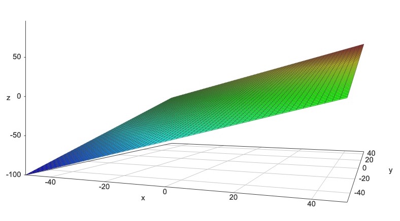
In the slope-intercept formula, substitute z for the dependent variable, fix the slope m at unity, and allow the intercept b to range independently as y.
A 3D plot of this formula appears as Figure 5. It's a plane which has constant slope in any direction.

Multiplication
In the slope-intercept formula, substitute z for the dependent variable, allow the slope m to range independently as y, and set the intercept b to zero.
A 3D plot of this formula appears as Figure 6. It's not a plane which has constant slope in any direction. Rather, it's a saddle shape. But the grid markings on the surface of this saddle are all straight lines. If you fix y as m then the function z = f(x) = mx plots as a straight line of slope m running through the origin, so f(x,y) is linear in x. Likewise if you fix x as m then the function z = f(y) = my plots as a straight line of slope m, again running through the origin. So f(x,y) is also linear in y.
Comments
- The fact that Isaac Newton invented the calculus earlier than Leibniz is not particularly relevant here. The functional underpinning developed by Leibniz to explain calculus—along with differential notation and the iconic cursive-S symbol for the integral—survive to animate introductory calculus courses in our present day. This page goes no further into calculus, although the topic of slopes is of great concern to calculus.
- My term “kinky” dances around the mathematical notion of differentiability.
| © Charles Ames | Page created: 2013-02-20 | Last updated: 2017-06-24 |