Demonstration 4
Markov Chaining
Introduction
Demonstration 4 provided the practical component for Chapter 6: “Conditional Selection I — Markov Chains” of my unpublished textbook on composing programs. It illustrates how Markov Chains can be employed to compose a piece of music. Markov chains are consistent with the selection pattern of G.M. Koenig's Project Two, to the extent that there is a sequence of events such as phrases or notes, and that even attributes such as duration and pitch are being drawn from a supply. In Markov's scenario, supply elements are called “states”, and there is an additional aspect of conditionality: The likelihood of selecting state i for event j depends on the state previously selected for event j-1.
The piece may be regarded as a chain of rhythmic units in the sense of “unit” used to explain Demonstration 2 and Demonstration 3.
Features of the Markov Matrix
A Markov transition matrix is a two-dimensional array of probabilities:
| p1,1 | p2,1 | … | pi,1 | … | pN,1 |
| p1,2 | p2,2 | … | pi,2 | … | pN,2 |
| ⋮ | ⋮ | ⋮ | ⋮ | ||
| p1,j | p2,j | … | pi,j | … | pN,j |
| ⋮ | ⋮ | ⋮ | ⋮ | ||
| p1,N | p2,N | … | pi,N | … | pN,N |
Where N is the number of states, where each pi,j ≥ 0, and where for each row of the matrix (that is, for each j),
The fact that each row sums to unity is why I use the term probability in favor of the less restrictive term weight.
Expanding from a one-dimensional distribution to a two-dimensional transition matrix adds a full order of complexity into the designer's task. Exercising control over the succession of choices means that among the multiplicity of available sequences, the matrix designer can use high probabilities to emphasize some sequences, use low probabilities to deemphasize other sequences, or use null probabilities to exclude still other sequences entirely.
Another feature is the ability to control the propensity for the chain to linger on one specific state. Such control is exercised through waiting probabilities, which are positioned along the diagonal of the matrix. Thus the waiting probability pi,i controls how often state i transitions to itself. Each waiting probability has an associated waiting count Ci,i. This waiting count gives the average number of times the chain will locally repeat state i before moving away. The two values pi,i and Ci,i have the following relationship:
|
|
Compositional Directives
The structure of Demonstration 4 is simpler than in previous demonstrations because there is no level of organization intervening between the individual notes and the piece as a whole. Each of the four attributes characterizing a unit — duration, articulation, register, and degree — proceeds independently of the others.
Articulation
Articulation is controlled through a percentage indicating the probability that an iteration of the composing loop will produce a note instead of a rest. There are four values: 10%, 17%, 29%, 50%. The waiting counts in each case will be 91%, which means the chain will linger upon one of these values for an average of
| 1 1-p |
= | 1 1-0.91 |
= 11.11 |
notes and rests before transitioning to a different state.
Transitions to new states emphasize the sequence 10% → 50% → 17% → 29% → 10%. On-track transitions have 5% probability, while off-track transitions have 2% probability. Since
the requirement of summing to unity is confirmed.
Average Note Duration
There are four average durations available to any note. Expressed in sixteenths, the averages for notes are D1=2, D2=3, D3=5, and D4=9; the averages for rests are half as much: 1, 1.5, 2.5, and 4.5.
Thus we can make each average duration persist over a whole-note duration by selecting Ci,i so that Ci,iDi=16, or
| pi,i = 1 - | Di 16 |
|
|
|
|
The waiting probabilities for all four values have been calculated so that the chain lingers on each value for approximately two measures before moving on to a new value. Table 1 illustrates how the average length over which a value holds sway may be computed as the product of the average duration itself and of the waiting count, which is the reciprocal of the waiting probability. We should recognize that control over how long an average duration holds sway is very loose, since both the waiting count and the individual durations are random. The number of random mechanisms affecting a process is often known as the degrees of freedom. The more degrees of freedom, the more the individual states of the process deviate from the norm.
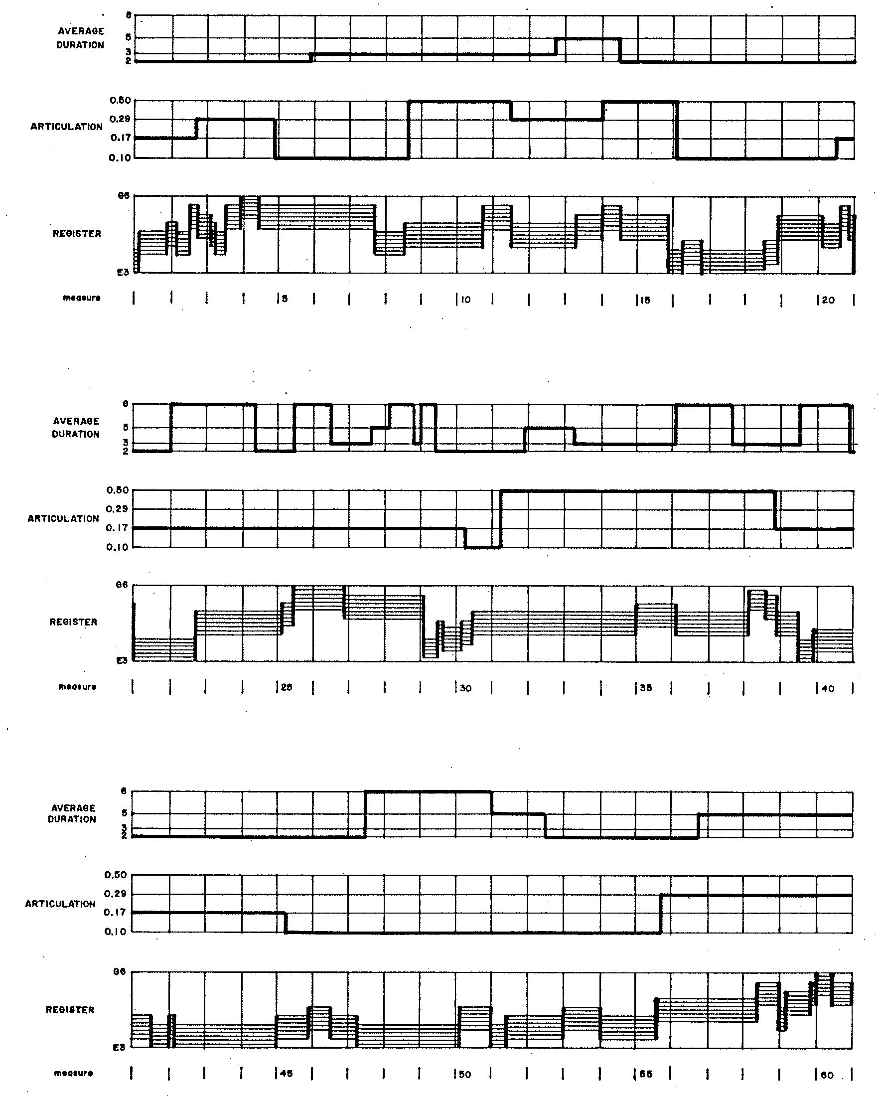
Figure 1 graphs the evolutions of average duration, articulation, and register in Demonstration 4. The rates of these evolutions directly result from the waiting probabilities controlling how individual states transition to themselves. Since waiting probabilities for articulations are high in Figure 1 (a), articulations evolve very slowly; by contrast, the waiting probabilities associated with the unison in Figure 1 (d)) are consistently zero, so no two consecutive notes repeat the same degree.
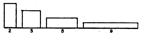
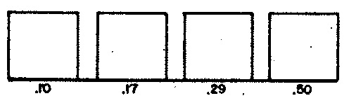
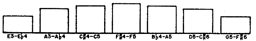
Also pertinent to the medium-term behavior are the stationary probabilities shown in Figures 2 (a-c). Stationary probabilities1 appear for average duration in Figure 2 (a); for articulation in Figure 2 (b); and for register in Figure 2 (c).
|
|
|
||
| Figure 2 (a): Stationary probabilities for average durations. | Figure 2 (b): Stationary probabilities for articulations. | Figure 2 (c): Stationary probabilities for registers. |
Register
Note Rhythms
The Markov chains controlling average note durations, articulations, and registers produced graphs which lingered for some numbers loop iterations before transitioning to the next value. This happened because the waiting probabilities — those located along the diagonal of the matrix — were nonzero. By comparison, the process used to decide whether a loop iteration should generate a note or a rest prescribes total certainty that a rest will never transition away to another rest but only a level of probability that a note will transition to another note. The process is in fact a two-state Markov chain, where the probability of transitioning from a note to another note is determined by the articulation percentage described above.
| Rest | Note | |
|---|---|---|
| Rest | 0 | 1 |
| Note | 1-p | p |
Table 1: Note/Rest transition matrix.
Note durations are selected according to the negative exponential distribution, but applying John Myhill's procedure to limit the ratio of maximum to minimum durations to 8.
Note Degrees
The progression of chromatic degrees reduces from a second-order Markov chain of chromatic positions to a first-order Markov chain of chromatic intervals. Figure 3 details the relative weights associated with each consecutive pair of intervals. Though intervals range from 1 to 11 (unisons are excluded), ‘wrap-around’ arithmetic keeps the current degree always within the range from 1 to 12.
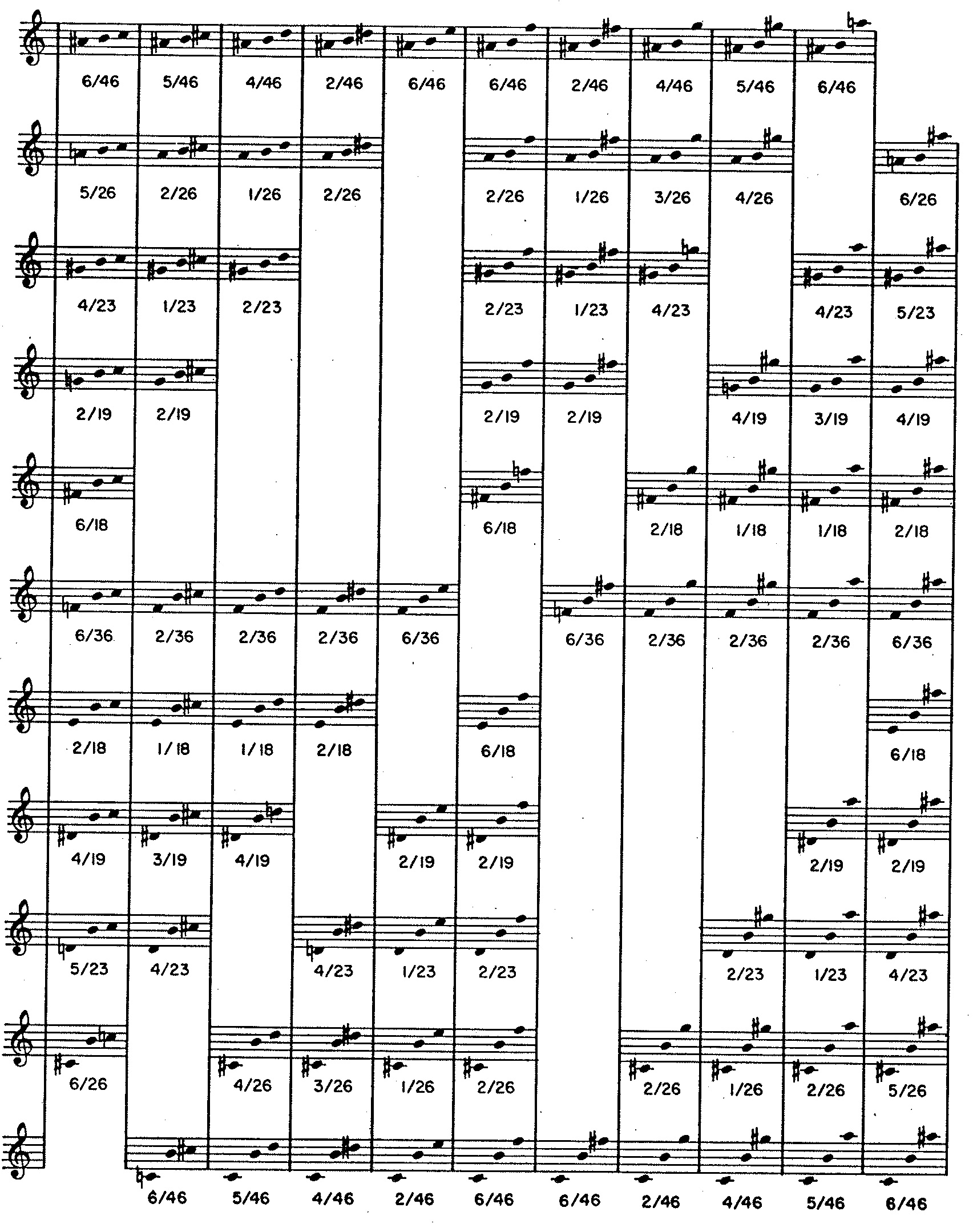
Figure 3: Stylistic matrix for Demonstration 4 — Each entry depicts a pair of two rising chromatic intervals with the middle degree fixed arbitrarily at B. The number of semitones in an interval corresponds to the extent of chromatic displacement.
The approach just described resembles the INTERVAL feature of G.M. Koenig's Project Two. Such matrices will be frequently employed in subsequent Demonstrations, where they will be designated as stylistic matrices. The current matrix acts both to enforce absolute constraints and to promote desirable tendencies, in this case to encourage a consistently dissonant style.
- Constraints are indicated by blank cells in Figure 3. Any triad containing chromatic identities (unisons, octaves) receives a weight of zero, as do major triads, minor triads, augmented triads, and triads with two perfect consonances (for example, C-F-Bb) in inversion or voicing.
- Second, the desirable tendencies: Of the non-blank cells in Figure 3, the numerator indicates the cell's relative weight, while the denominator indicates the row total. Relative weights range from 1 to 6, favoring dissonance. Thus, triads combining a perfect fifth with a minor seventh (for example, C-G-Bb) always receive a relative weight of 1, regardless of inversion. Triads combining a tritone with a major seventh (for example, C-F#-B) or combining two semitones (for example, C-C#-D) always receive a relative weight of 6.
The language of constraints is inherently dogmatic. Practices are either correct or incorrect. Just bear in mind that the dogma applies only to this particular composing program. These Demonstrations in no way suggest that adherence to universal standards will improve the quality of your music. Artusi lost that argument to Monteverdi centuries ago. Rather, the take-away lesson from these Demonstrations is that if there certain patterns run contrary to the style your program is intended to generate, and if you are able to formulate constraints forbidding these patterns, then there are methods which you can use to enforce such constraints, that some methods are more efficient than others, and that where these methods occur in the decision-making logic can also make a difference.
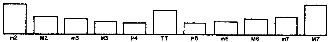
Stationary probabilities calculated from Figure 3 appear in Figure 4.
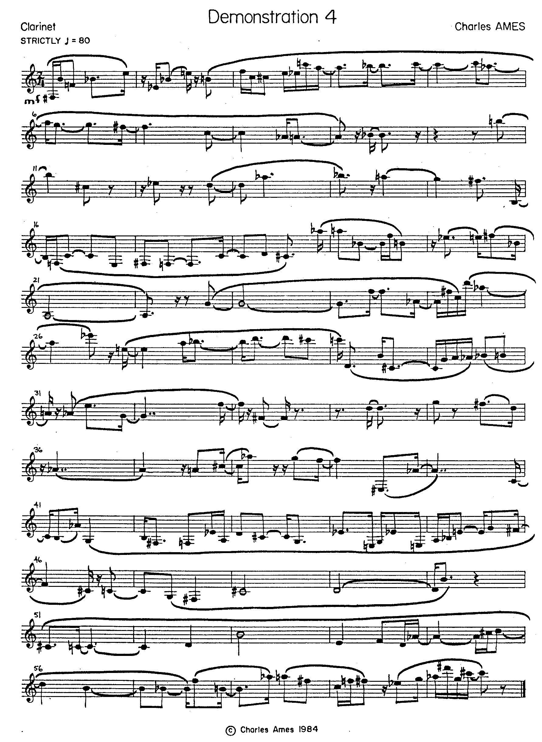
A transcription of the musical product appears in Figure 5.
Implementation
The explanations to follow focus variously on four attributes of musical texture: average note duration, articulation, register, and chromatic degree. The purpose is to tease out the strands of code that affect a particular attribute, and thus to illustrate Markov chaining in play. The explanations are peppered with line numbers, but you are are by no means expected to chase down every line of code. Rather, you should follow through with line numbers only when you have a specific question that the narrative is not answering.
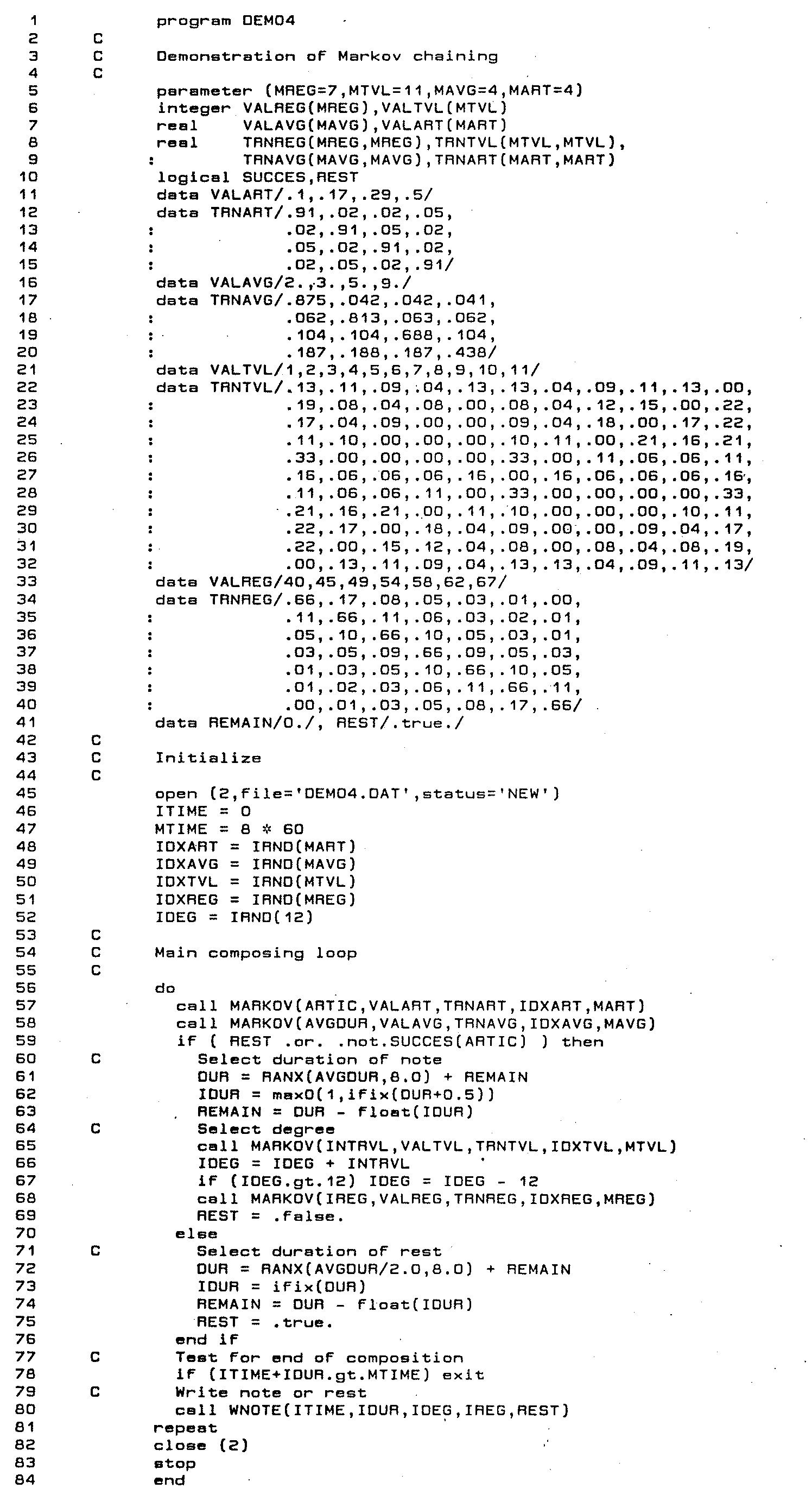
The source code for program DEMO4 appears as Listing 1.
This program implements the one-tiered structure described above as a single
composing loop (lines 56-81) which iterates for each note or rest and which continues until sixty measures
of 2/4 time have been filled out (line 78). At the beginning of an iteration, the program chooses an average duration, expressed
in sixteenths, and a rest/play probability. Line 59 executes a random branch to determine whether to compose a note
(lines 61-69) or a rest (lines 71-75).
Average Note Duration
Variables and arrays pertaining to average duration of notes (equivalently, average tempo) have names ending with AVG.
The average duration of rests is half as large.
-
Parameter
MAVGfixes the number of average note durations at 4 (line 5); line 16 populates specific values into arrayVALAVG. The integer variableIDXAVGtracks the current state of the average-duration chain. -
Lines 17-20 populate the
MAVG×MAVGarrayTRNAVGwith transition probabilities. Stationary probabilities derived from this matrix are shown in Figure 2 (a). -
Line 49 initializes index
IDXAVGwith uniform randomness by calling the library functionIRND. -
Moving down into the note/rest loop, line 58's call to subroutine
MARKOVexecutes the next transition in the average-duration chain, reselectingIDXAVGand then dereferencingVALAVG(IDXAVG)into the variableAVGDUR. The values selected forAVGDURare shown in the uppermost graph of Figure 1. -
Specific note durations are generated in line 61, where variable
AVGDURbecomes the first argument in a call to the library function RANX. Rest durations are generated similarly in line 72, except that here the value ofAVGDURis scaled down by half.
Articulation
Variables and arrays pertaining to articulation have names ending with ART.
Articulations are expressed as the probability that a rhythmic unit will serve as a rest.
-
Parameter
MARTfixes the number of articulation-probabilities at 4 (line 5); line 11 populates specific values into arrayVALART. The integer variableIDXARTtracks the current state of the articulation chain. -
Lines 12-15 populate the
MART×MARTarrayTRNARTwith transition probabilities. Stationary probabilities derived from this matrix are shown in Figure 2 (b). -
Line 48 initializes index
IDXARTwith uniform randomness by calling the library functionIRND. -
Moving down into the note/rest loop, line 57's call to subroutine
MARKOVexecutes the next transition in the articulation chain, reselectingIDXARTand then dereferencingVALART(IDXART)into the variableARTIC. The values selected forARTICare shown in the central graph of Figure 1. -
Remember that the question of whether a loop iteration should generate a note or a rest is controlled by the two-state transition
matrix given in Table 1, where the probability p that a note will transition
into another note corresponds to the variable
ARTIC.2. In line 59, the variableRESTdetermines whether row 1 (Rest) or row 2 (Note) of Table 1 applies. IfRESTis true, then the choice becomes determinate: generate a note. Otherwise, a call to functionSUCCESsettles the note/rest decision through a Bernoulli trial.
Register
Variables and arrays pertaining to register have names ending with REG.
Registers are expressed as the lowest position in a twelve-semitone gamut.
-
Parameter
MREGfixes the number of registral gamuts at 7 (line 5); line 33 populates specific values into arrayVALREG. The integer variableIDXREGtracks the current state of the register chain. -
Lines 34-40 populate the
MREG×MREGarrayTRNREGwith transition probabilities. Stationary probabilities derived from this matrix are shown in Figure 2 (c). -
Line 51 initializes index
IDXREGwith uniform randomness by calling the library functionIRND. -
Moving down into the note/rest loop, line 68's call to subroutine
MARKOVexecutes the next transition in the register chain, reselectingIDXREGand then dereferencingVALREG(IDXREG)into the variableIREG. The values selected forIREGare shown in the lowermost graph of Figure 1. This variable is consumed in line 80 with a the call toWNOTE.
Chroma
Variables and arrays pertaining to chromatic intervals have names ending with TVL.
Chromatic intervals are expressed as integers from 1 (minor second) to 11 (major seventh).
-
Parameter
MTVLfixes the number of intervals at 11 (line 5); line 21 populates specific values into arrayVALTVL. This redundant setup is done for compatibility with subroutineMARKOV. The integer variableIDXTVLtracks the current state of the register chain. -
Lines 22-32 populate the
MTVL×MTVLarrayTRNTVLwith the transition probabilities detailed in Figure 4. Stationary probabilities derived from this matrix are shown in Figure 2 (d). -
Line 48 initializes index
IDXTVLwith uniform randomness by calling the library functionIRND. -
Moving down into the note/rest loop, line 57's call to library subroutine
MARKOVexecutes the next transition in the register chain, reselectingIDXTVLand then dereferencingVALTVL(IDXTVL)into the variableITVL. This variable is wrapped into the range from 1 to 11 and consumed in line 80 with a the call toWNOTE.
The loop completes in line 80 with a call to subroutine WNOTE. This version of WNOTE takes as argument #5
the note/rest flag REST. If REST is true, register (argument #3) and degree (argument #4) are ignored.
If REST is false, WNOTE uses the library subroutine IOCT
to place IDEG in the register indicated by IREG.
Executing a Markov Transition
The library subroutine MARKOV3 implements random
selection with probabilities conditioned by previous choices.
Calls to MARKOV require five arguments:
-
RESULT—MARKOVselects a state (supply value) and returns the value in this location. -
VALUE— Supply of state values. Duplicate values are not permitted.VALUEmust be an array whose dimension in the calling program isNUM(argument #5 below). -
TRANS— Array of transition probabilities. Trans must be a real array in the calling program whose duration isNUMbyNUM. The probabilities must be non-negative, and every row of the array must sum to unity. -
IDX— Index to previously-selected state.IDXmust be an integer in the calling program. This argument provides the element of feedback. Since FORTRAN passes subroutine arguments by address, each call toMARKOVupdates variableIDXto the newly selected state. -
NUM— Number of states.NUMmust be an integer in the calling program.
MARKOV first calculates a row offset I=NUM*(IDX-1). This means that the
upcoming state selection will be governed by the probabilities TRANS(I+1), TRANS(I+1), …
TRANS(I+NUM). According to the restrictions given for array TRANS above, these probabilities
must sum to unity. MARKOV then uses the methods of the library subroutine
SELECT to select the new value of IDX, where the
‘chooser’ value R= is unscaled. MARKOV completes by setting RESULT=VALUE(IDX).
Comments
- The procedure for calculating stationary probabilities is explained in Automated Composition, Chapter 6, pp. 6-8 to 6-9.
- Understand that the note/rest mechanism for Demonstration 3 essentially matches what happened both in Demonstration 2 and Demonstration 3. These previous implementations were in fact doing Markov chains for this particular mechanism.
-
Subroutine
MARKOVis presented in Automated Composition, Chapter 6, pp. 6-16 to 6-18.
| © Charles Ames | Original Text: 1984-11-01 | Page created: 2017-03-12 | Last updated: 2017-03-12 |