Demonstration 6
Evolutions

Introduction

Demonstration 6 provided the practical component for Chapter 8: “Musical Design I — Evolutions” of my unpublished textbook on composing programs. It illustrates how evolutions might be used in a composing program. The piece divides into eight segments, within which the following four global attributes gradually change: average period, proportion between minimum and maximum periods (syncopation), articulation, and register. The eight segments in turn divide into individual notes, each characterized by three local attributes: period, duration, and pitch.

Compositional Directives

Figure 1 depicts graphically how the global attributes evolve.

Both the average period and the proportion between minimum and maximum periods are described by piecewise exponential curves.

The method of selecting articulations is adapted from the TENDENCY feature of Gottfried Michael Koenig's Project Two. An evolving mask carves out portions from a region of uniform probability. This region divides into four equal-sized sub-regions (indicated by horizontal hairlines in the third-from-top graph in Figure 1).

1. Short — duration fills 50% of period,
2. Detached — duration fills 75% of period,
3. Sustained — duration fills entire period, but next note is tongued, and.
4. Slurred — duration fill entire period and next note is slurred.

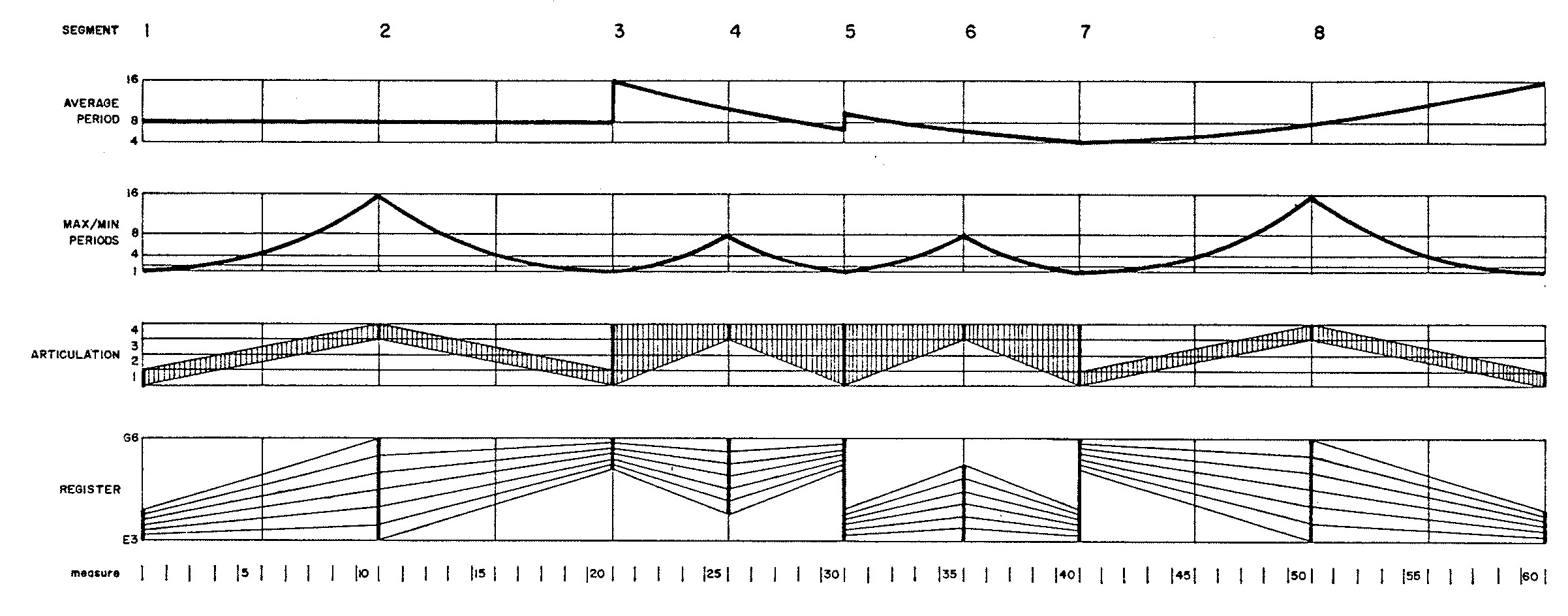
Registers are determined by located a gamut of twelve adjacent semitones uniformly within the lower and upper and upper boundaries depicted in the registral graph.

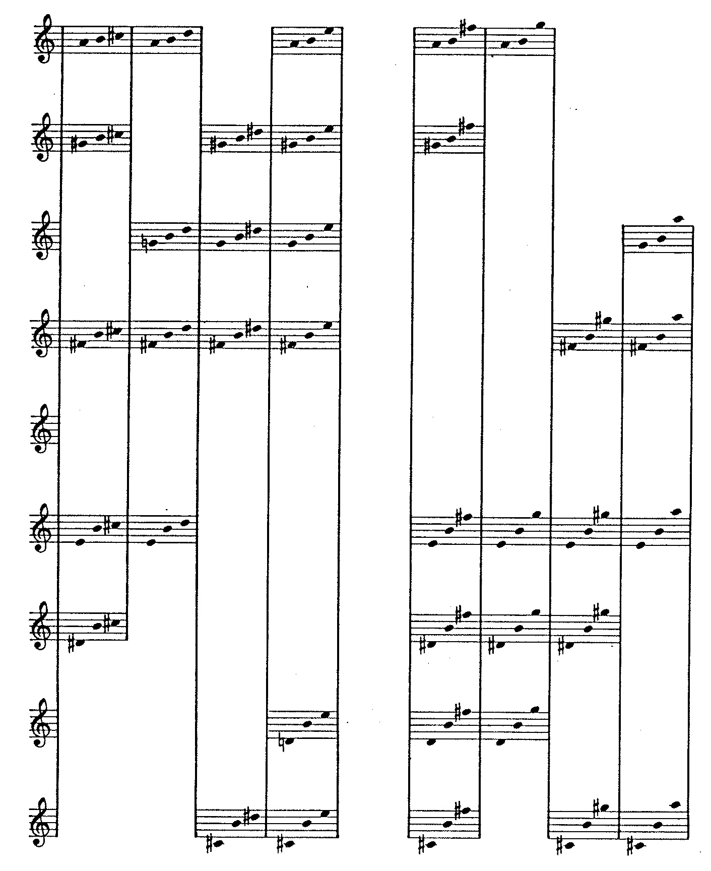
Of the local attributes, periods are selected in accordance with the average period and maximum proportion using John Myhill's generalization of the exponential distribution. Durations are calculated from the period in accordance with the articulation. Chromatic degrees are selected using cumulative feedback so that the twelve degrees are equally balanced with sensitivity to duration. However, choices of degrees are subject to the stylistic matrix depicted in Figure 2. This matrix constrains the progression of degrees so that no two out of any three consecutive degrees may form a unison, tritone, minor second, or major seventh. Neither may such degrees form expansions of any of the proceeding intervals by one or more octaves.

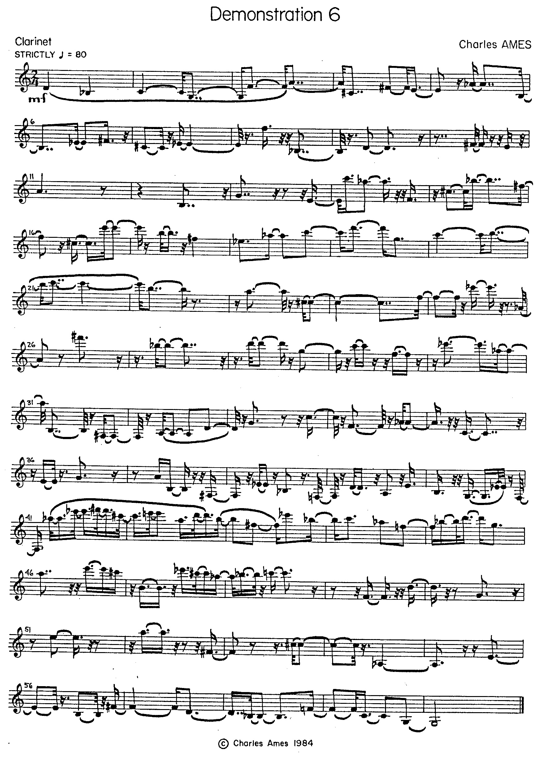
The transcribed product appears in Figure 3.

Implementation

The explanations to follow focus variously on four attributes attributes of musical texture which evolve gradually over time. The purpose is to tease out the strands of code that affect a particular attribute, and thus to reveal evolutionary calculations in play. The explanations are peppered with line numbers, but you are are by no means expected to chase down every line of code. Rather, you should follow through with line numbers only when you have a specific question that the narrative is not answering.

Program DEMO6 is reproduced in Listing 1. Because the global structure of Demonstration 6 is fully specified, program DEMO6 reduces to a single loop for composing notes (lines 35-86). The evolutions in Figure 1 divide into eight segments whose start and end times are shared in common between the various musical attributes depicted in the graph. The declaration of parameter MSEG in line 5 fixes the total number of segments at 8. Array KTIME holds ending times for each segment; these times are initially expressed in seconds, so must be converted to thirty-second notes (lines 29-33).

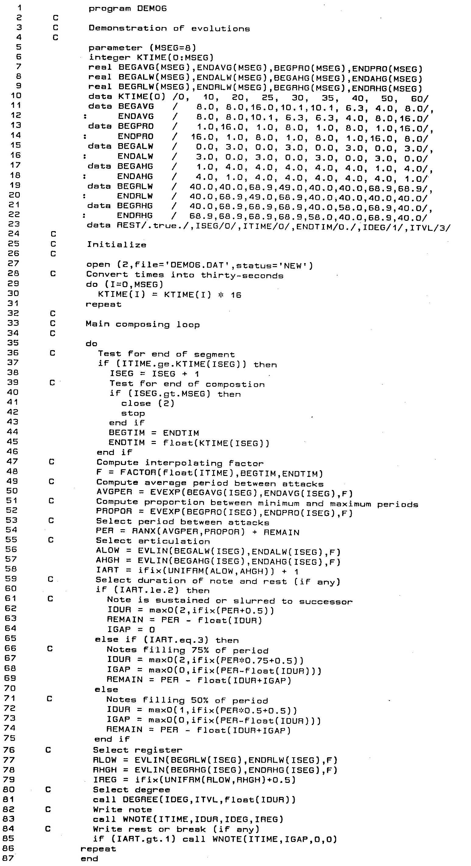
The index ISEG indicates which segment the program is currently composing. Lines 37-46 serve to update ISEG whenever the current time ITIME (initialized to zero in line 23) crosses a boundary between segments. Included here is the test for completion (lines 40-43). This change in ISEG shifts the previous segment's ENDTIM into the current segment's BEGTIM (line 44), then dereferences the current segment's end time FLOAT(KTIME(ISEG)) into the simple variable ENDTIM (line 45).

The call to the library function FACTOR in line 48 calculates a single interpolation factor as of ITIME for all musical attributes controlled by evolutions. This interpolation factor is stored in the simple real variable F. The evolving musical attributes are identified by the following symbolic abbreviations:

Rhythm

Rhythm in Demonstration 6 conflates three of the musical attributes graphed in Figure 1. The period between consecutive attacks is controlled by the average period and by the max/min proportion. The sounding duration of individual notes is determined by the articulation.

Variable names containing the abbreviation PER — pertain to periods between note-attacks. This note-specific attribute is generated in line 54 by a call to the library function RANX, originally introduced in connection with Demonstration 2. Here we see the function employed as John Myhill intended it to be used. Arguments to this function call are supplied by two simple variables: AVGPER is the average period length (equivalently, average tempo); this is the quantity plotted in the topmost graph of Figure 1. PROPOR is the proportion between maximum and minimum values (‘syncopation’); this is the quantity plotted in the second-from-top graph of Figure 1. We now trace how AVGPER and in turn PROPOR are calculated.

• Array elements BEGAVG(ISEG) and ENDAVG(ISEG) hold the beginning average period and ending average period, respectively, for segment number ISEG. These arrays are declared in line 7 and populated in lines 11-12. The momentary average period as of ITIME is calculated by a call to the library function EVEXP in line 50, making use of the interpolation factor F calculated in line 48. The result is stored in AVGPER.
• Array elements BEGPRO(ISEG) and ENDPRO(ISEG) hold the beginning proportion and ending proportion, respectively, for segment number ISEG. Understand that this second parameter to RANX can range upward from unity, which indicates strictly period rhythm. Values above 1000 produce pure negative exponential randomness, but I have elected here to employ an upper limit of 16. The BEGPRO and ENDPRO arrays are declared in line 7 and populated in lines 13-14. The momentary average period as of ITIME is calculated by a call to the library function EVEXP in line 52, making use of the interpolation factor F calculated in line 48. The result is stored in PROPOR.

Articulation in Demonstration 6 influences how the period between consecutive attacks divides into two components: the sounding duration of the note and the gap of silence between the current note's release and the upcoming note's attack. Four modes of undertaking this division were explained above: short, detached, sustained, and slurred. The mode of division is selected by generating a chooser value in the range from 0.0 to 4.0, then rounding the chooser up to the next integer. However only, a portion of this total range is actually used to generate the chooser, and that portion is determined by an evolving “mask” (Koenig's term).

• Array elements BEGALW(ISEG) and ENDALW(ISEG) hold the beginning and ending lower bounds, respectively, of the mask used to select an articulation during segment number ISEG. These arrays are declared in line 8 and populated in lines 15-16. The lower mask bound as of ITIME is calculated by a call to the library function EVLIN in line 56, making use of the interpolation factor F calculated in line 48. This lower mask bound is stored in the simple variable ALOW.
• Array elements BEGAHG(ISEG) and ENDAHG(ISEG) hold the beginning and ending higher bounds, respectively, of the mask used to select an articulation during segment number ISEG. These arrays are declared in line 8 and populated in lines 17-18. The higher mask bound as of ITIME is calculated by a call to the library function EVLIN in line 56, again making use of F. This higher mask bound is stored in the simple variable AHGH.

The mode of articulation IART is selected by the expression IFIX(UNIFRM(ALOW,AHGH))+1 in line 58.

Pitch

Pitch in Demonstration 6 conflates the fourth musical attribute graphed in Figure 1, register, with a chromatic degree selected using the method employed previously in Demonstration 5. This method subjects cumulative feedback to constraints.

First to register:

• Array elements BEGRLW(ISEG) and ENDRLW(ISEG) hold the beginning and ending lower bounds, respectively, for registers during segment number ISEG. These arrays are declared in line 9 and populated in lines 15-16. Values in these two arrays range from 40, corresponding to E3, the lowest pitch on the clarinet, upwards to 68.9. This higher value corresponds roughly to Ab5, which when combined with a degree can produce pitches up to G6. The lowest register as of ITIME is calculated by a call to the library function EVLIN in line 77, making use of the interpolation factor F calculated in line 48. This lowest register is stored in the simple variable RLOW.
• Array elements BEGRHG(ISEG) and ENDRHG(ISEG) hold the beginning and ending higher bounds, respectively, for registers during segment number ISEG. These arrays are declared in line 9 and populated in lines 17-18. Values again range E3 to roughly Ab5, though the register graph in Figure 1 is adjusted to include the additional octave contributed by degree selection. The highest register as of ITIME is calculated by a call to the library function EVLIN in line 78, again making use of F. This highest register is stored in the simple variable RHGH.

The specific register IREG is selected by the expression IFIX(UNIFRM(RLOW,RHGH)+0.5) in line 79. This value fixes the bottom of a twelve-semitone gamut within which a chromatic degree will be placed.

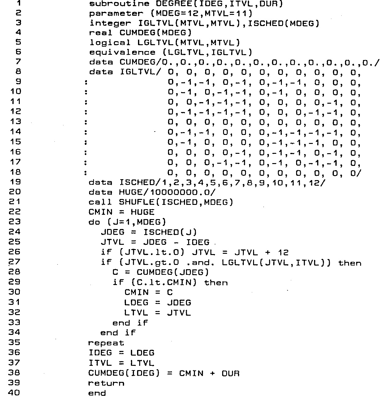
Line 81 of program DEMO06 delegates the task of selecting a chromatic degree to subroutine DEGREE. The source code for subroutine DEGREE code appears in Listing 2.

The declaration of parameter MDEG in line 2 fixes the number of chromatic degrees at 12. Facts about degrees are maintained in array ISCHED and array CUMDEG. ISCHED provides an indirect schedule of chromatic numbers. It is declared in line 3 and populated in line 19 with the integers 1-12. CUMDEG maintains usage statistics for each degree instance. It is declared in line 3 and populated entirely by zeros (indicating no usage so far) in line 7. There is no array of weights corresponding to CUMDEG; this omission is due to the fact that the twelve chromatic degrees have uniform weight.

The declaration of parameter MTVL in line 2 fixes the number of chromatic intervals (excluding the unison) at 11. Constraints affecting pairs of consecutive intervals are itemized in the 11×11 logical array LGLTVL which implements the constraint matrix depicted as Figure 2. LGLTVL is declared in line 5 and populated in lines 8-18 where the integer value 0 corresponds to the truth value .FALSE. (all bits cleared) and the integer value -1 corresponds to the truth value .TRUE. (all bits set). This sleight of hand — data entering brief numbers rather than cumbersome truth values — is accomplished in line 6 by establishing an EQUIVALENCE between the logical array LGLTVL and the 11×11 integer array IGLTVL.

Calls to subroutine DEGREE require three arguments:

1. IDEG — An integer ranging from 1 to 12. Coming into subroutine DEGREE, this variable holds the previously selected degree. Returning from subroutine DEGREE, this variable holds the newly selected degree.
2. ITVL — An integer ranging from 1 to 11 (unisons are excluded). Coming into subroutine DEGREE, this variable holds the chromatic interval by which the previously selected degree was approached. Returning from subroutine DEGREE, this variable holds the chromatic interval from the old value of IDEG to the new value of IDEG.
3. DUR — Sounding duration of the current note, in thirty-second notes.

Subroutine DEGREE seeks to identify a chromatic degree IDEG for which the statistic CUMDEG(IDEG) is minimal while at the same time satisfying the intervallic constraints itemized in matrix LGLTVL. It does so with the following steps.

1. Line 21 randomly shuffles array ISCHED into random order; this eliminates any bias which might result from how chromatic degrees are enumerated.
2. Variable LDEG identifies the chromatic degree which satisfies all constraints and which possesses the smallest CUMDEG value discovered so far, which value is recorded in variable CMIN. Variable LTVL calculates the interval from IDEG to LDEG. Upon entering subroutine DEGREE, CMIN is set very large while both LDEG and LTVL are indeterminate.
3. The loop implemented in lines 22-35 iterates through chromatic degrees in the order determined by array ISCHED. The loop indexes on variable J. Each iteration begins by dereferencing ISCHED(J) into the simple variable JDEG, thus JDEG is the candidate currently being considered. The interval from IDEG to JDEG is calculated into variable JTVL.
4. Line 27 evaluates JTVL. If JTVL is a unison (JTVL = 0) or if the constraint matrix is unsatisfied (LGLTVL(ITVL,JTVL) evaluates .FALSE.) then the candidate JDEG is rejected and the loop proceeds to the next iteration.
5. If JTVL ≠ 0 and the constraint matrix is satisfied (LGLTVL(ITVL,JTVL) evaluates .TRUE.) then
   1. Line 29 compares the candidate statistic CUMDEG(JDEG) to the best-yet-discovered statistic CMIN.
   2. If CUMDEG(JDEG) < CMIN then CUMDEG(JDEG) overwrites CMIN, JDEG overwrites LDEG, and JTVL overwrites LTVL (lines 30-32).
6. Line 38 increments CUMDEG(IDEG) by DUR.

Resuming now with program DEMO06, the chromatic degree IDEG returned from line 81's call to subroutine DEGREE is marshaled together with the current time ITIME, the note duration IDUR, and the register IREG. Line 83 passes these combined facts to the note-writing subroutine WNOTE. A second call to WNOTE happens in line 85 if the note duration falls short of the period between consecutive attacks. That completes the current iteration of the note-generating loop.

Computing an Interpolation Factor

The process of computing an intermediate value given a start time, end time, origin, and goal is called interpolation. Both linear and exponential interpolations depend upon the ratio of the elapsed time to the entire segment duration. This ratio is called the interpolating factor. In cases where an item within one segment draws upon several concerted evolutions, it becomes redundant to recompute this factor for each evolution. The real-valued library function FACTOR¹ isolates the mechanics of computing an interpolation factor. FACTOR require three real arguments:

1. T — current time.
2. TA — Segment start time. TA must not exceed T.
3. TB — Segment end time. T must not exceed TB.

Given these three values, FACTOR returns the quotient (T-TA)/(TB-TA).

Calculating a Linear Interpolation

The real-valued library function EVLIN¹ computes values along linear contours. EVLIN require three real arguments:

1. A — origin value of contour at beginning of segment.
2. B — goal value of contour at end of segment.
3. F — Interpolating factor (provided by the library function FACTOR).

Given these three values, EVLIN calculates the result A + (B-A)*F.

Calculating an Exponential Interpolation

The real-valued library function EVEXP¹ computes values along exponential curves. EVEXP require three real arguments:

1. A — origin value of contour at beginning of segment. Must be positive.
2. B — goal value of contour at end of segment. Must be positive.
3. F — Interpolating factor (provided by the library function FACTOR).

The value EVEXP returns depends upon how A compares to B.

• If A ≈ B — then EVEXP returns A.
• If A < B — then EVEXP returns A*(B/A)**F.
• If A > B — then EVEXP returns B*(A/B)**(1-F).

Where the double asterisk ** is FORTRAN's exponentiation operator.

Comments

1. The static, array-based implementation employed for these Demonstrations gave way in later work to a dynamically allocated framework of contours pieced together from segments. For example the ASHTON score-transcription utility employed contour frameworks to represent tempo, dynamics, and custom parameter evolutions. The FORTRAN source code for functions FACTOR, EVLIN and EVEXP appears in Automated Composition, Chapter 8, pp. 8-6 to 8-7.