Sound Engine Basics
Introduction
MUSIC-N was a series of digital-sound-synthesis programs
developed during the 1960's by Max Mathews with colleagues Joan E. Miller,
F. R. Moore, John R. Pierce, and
J. C. Risset
at Bell Telephone Laboratories.
The fifth and last of the Bell Labs programs was described in a famous book,
The Technology of Computer Music.
The MUSIC-N programs sought to emulate analog components of the
classical electronic music studio, e.g.
oscillators,
noise generators,
envelope generators, and
filters.
Ultimately the digital technology represented by MUSIC-N doomed analog technology to obsolescence.
To many people, non-real time software synthesis has itself been rendered obsolete by real-time digital synthesis hardware. However to someone with low-grade performance skills (such as myself), whether or not a sound has been generated in real time is not particularly important. Software synthesis presents many opportunities. Foremost is the ability to shape sound on its most elemental level. Even if one never wishes to realize compositions, this ability gives one direct involvement with sound that Helmholtz would have killed for. Beyond this, software syntheses allows one to sculpt sounds of arbitrary complexity — without limits on the number of simultaneous tones and without concern that calculations execute quickly enough to keep up with digital-to-analog conversion.
I personally worked with Stanford's music system during a summer workshop in 1976 and with Barry Vercoe's Music11 (a
precursor to CSound) during a summer workshop at M.I.T. in 1978. MUSIC-V was in use at the State University of New York
at Buffalo (UB) when I began graduate studies there in 1977. After the M.I.T. workshop I tried to persuade Hiller to adopt Music11
but Vercoe wanted to charge license fees and Hiller would have none of that. I subsequently began working up my own Sound program with
some of the capabilities I had witnessed elsewhere; for example, dynamic memory allocation, constants and variables in instrument definitions,
and greater unit diversity. This program was actually generating wave files when a flood came through and destroyed UB's primitive
digital-to-analog conversion facility. The Sound application presently described on this site recasts that original program
for the desktop computer.
Things have changed since the 1970's. UB's CDC 6600, designed by Seymour Cray and a “supercomputer” of its day, is today dwarfed in both speed and memory capacity by common desktop units. Those same desktops have sound cards with high-speed, high-resolution, digital-to-analog and analog-to-digital conversion. Proprietary audio files have given way to standardized WAV and MP3 formats. Specialized component-description “languages” are now superseded by XML. And of course the internet, which was barely getting started in those days, is now ubiquitous.
Overview
The text that follows first sets the context by explaining the distinction between additive synthesis and subtractive synthesis. It then gets down to brass tacks by describing the WAV format used to contain an audio signal. The text proceeds to walk through how a sound-synthesis engine would use the simplest instrument and a one-note score (i.e. notelist) to generate an audio signal. Essential to this is the operation of the digital oscillator and how it contends with quantization noise and foldover. Returning to the engine, the text explains how audio-rate calculations combine signals from instruments and buffer up results for file output. It then describes note initialization, a feature of the post-Bell-Labs generation of sound-synthesis packages. Finally, the text explains voices, contours, and ramps, which are unique features (so far as I know) of my own Sound engine.
Sound-Synthesis Models
The years following World War II combined a new experimental spirit — responding in part to years of cultural suppression in Europe — with an enthusiasm for the wondrous new technologies that had been so stimulated by the war effort. These impulses spawned two approaches to what we now know as electro-acoustic music:
- Musique concrète or “tape-music” is associated with Pierre Schaeffer and Pierre Henry of the Office de Radiodiffusion-Télévision in Paris. This approach, alternatively known in English as “tape music”, featured environmental sounds captured using the new-fangled tape recorder and combined together by mixing and splicing in the studio.
- Pure electronic music was pioneered by Herbert Eimert and Werner Meyer-Eppler, who together founded the electronic music studio at Nordwestdeutscher Rundfunk in Cologne. This latter approach combined additive synthesis, that is, building up complex sounds from simple tones generated by an oscillator, with subtractive synthesis, which begins with complex noise sounds and shapes them using filters.
Mixing and splicing are pervasive in electro-acoustic music today, though what was once done using tape segments is now done using digital wave files. What Schaeffer and Henry did to incorporate environmental sounds has evolved into the general technique of sampling. The idea of recreating instrumental sounds by separately recording individual tones and playing them back on cue has been around since the mellotron, a 1963 instrument which employed a different tape loop for every tone on its keyboard. Digitizing this concept produced sampling synthesizers; these evidently existed as early as 1967 but did not really take off until the mid 1980's.
A particular technique of tape music as been the use of tape loops to create an echo effect. With the advent of digital delay, what was originally an expensive, noise-prone, and inflexible effect became the basis of a new frontier in digital sound synthesis and digital signal processing. An early application of digital delay was artificial reverberation, as described in a famous article by Manfred R. Schroeder. However it was also realized that if one processed an impulse (e.g. a noise source) through a delay line with a very short loop time, then the delay line would resonate harmonically like the tube of a clarinet or a string on a violin. Such is the basis of the plucked string technique developed by Karplus and Strong sometime before 1981.
Additive synthesis builds toward complexity by adding sine waves together, each with a particular amplitude. In rudimentary additive synthesis, amplitudes are static; that is, they remain fixed over the duration of a sound. When the sine waves are tuned according to the harmonic series, the result is a periodic waveform. Static waveforms are the subject of my page on Oscillators and Waveforms. In advanced additive synthesis, the amplitude of each harmonic changes dynamically over time. More on additive synthesis may be found in Wikipedia.
Subtractive synthesis begins with broad-spectrum sounds like noises and pulse waves. It then employs filters to selectively enhance or degrade specific regions of the sound spectrum. In the early days of electronic music, “subtractive synthesis” specifically referred to ways of filtering the output from a noise generator, and this is the topic of my page on Synthesizing Noise Sounds. However, researchers in speech synthesis during the same time, notably Gunnar Fant, concluded that a source-filter model contributed strongly to the understanding of speech sounds. Acousticians have since applied the source-filter model directly to the production of musical tones; for example to how the resonant body of stringed instruments affects the tones of these instruments, or how the shape of the air column (cylindrical in trumpets or conical in horns) affects the production of brass tones. The Wikipedia article on subtractive synthesis unfortunately provides less information than I have given here.
The distinction between additive and subtractive methods has long been useful as a way of organizing sound synthesis techniques in the minds of new students. These have never been doctrines championed by one side or another. Yet in comparing the summer workshop I attended at Stanford in 1976 with the workshop I attended at M.I.T. in 1978, the difference in emphasis fell out along this distinction. I should say before I launch into this narrative that the contrast probably had less to do with institutional philosophies and more to do with the fact that the Standford workshop targeted beginners, while the M.I.T. workshop targeted experienced teachers.
Additive Synthesis at Stanford in 1976
Stanford's 1976 summer workshop on Computer-Generated Sound lasted only four weeks, but provided the most exhilarating experience of my entire life. Fellow attendees at Stanford included Larry Polansky, Neil Rolnick, and Beverly Grigsby.
At Stanford the presenters assumed we had no previous experience with computer sound synthesis — certainly true in my case —
and therefore started us out with the basics. Presenters included F. Richard Moore on the workings
of MUSIC-N-style sound synthesis,
Leland Smith on score preparation, John M. Grey (a Ph.D. candidate in Stanford's psychology
department) on psycho-acoustics, John Chowning on advanced topics.
Loren Rush was also on staff; I don't remember him formally presenting but he
did give out encouragement.
Dick Moore explained the fundamental sound-generating units with particular emphasis on the digital oscillator.
Meanwhile Leland Smith explained how to create simple note lists
(they called them “score files”).
To try things out, we were initially given an instrument named SIMP which consisted of a single oscillator generating
a sine wave. Having no envelope, notes generated by SIMP started and ended with obnoxious clicks.
This problem was shortly remedied with a second instrument design where one oscillator generated a one-cycle ADSR envelope which
drove the amplitude of a second audio-frequency oscillator. This second design was employed by four instruments whose sole
difference was the waveform sampled by the audio-frequency oscillator: TOOT sampled a sine wave.
CLAR sampled a square wave. BUZZ sampled a pulse wave.
BRIT sampled a sawtooth wave.
These four sounds provided the basis for an extended tape composition by Beverly Grigsby. Moore and Smith must have told
us about the random noise generator because I used it for my own project, a piece for synthesized percussion.
I don't remember any mention of digital filtering during these sessions.
Of Grey's lectures on psycho-acoustics I remember a specific focus on the studies performed by Reiner Plomp and Willem Levelt. Much of Plomp and Levelt's work concerned on the perception of sine-tone interactions within and outside the Critical Band, and this concern with sine waves is very consistent with the additive outlook.
I believe it was John Grey who played us the example of instrument tones morphing between four instruments. Here my memory fails me. I remember two of the instruments definitely being trumpet and violin. A third might have been the oboe. I don't remember the fourth at all. In any case, this demonstration showed off the additive model in its full dynamic glory, since it was achieved by obtaining amplitude envelopes for each harmonic of each instrumental tone, and then using interpolation techniques to transform each envelope of one instrument into the corresponding envelope for a second instrument.
The advanced topics presented by John Chowing included FM synthesis and the synthesis of moving sounds. Details about FM synthesis may be found in Chowning's excellent article. All I want to point out here is that Chowning's method provides a shortcut to producing tones with dynamically evolving spectra, meaning that the amplitude of each harmonic changes constantly over the duration of a note. In my mind, this aligns FM synthesis firmly on the additive side of the additive-subtractive dichotomy. As for Chowning's synthesis of moving sounds, I had already witnessed that a few months earlier. On that previous occasion, the California Institute of the Arts hosted a one-day computer-music symposium. Chowning was there, as were other presenters whose names I have long since forgotten. These other presenters were up first. They proudly demonstrated a system that could direct each single note to any one of eight (even 32, they speculated) speakers located around the room. Chowning came up next, and using 4 speakers, produced a single continuous sound that whizzed around the room — enhanced even by a Doppler effect.
Subtractive Synthesis at M.I.T. in 1978
After Stanford, I wasn't greatly convinced there was much more to learn about computer sound synthesis. When I attended the 1978 summer workshop at M.I.T., I'd only vaguely heard the name of Barry Vercoe. The main attractions of the workshop were first to regain access to a top-rate sound-synthesis facility and second to take advantage of the second session, during which attendees could pursue compositional projects. Fellow attendees at M.I.T. included Larry Austin, William Benjamin, Robert Ceely, Alexander Brinkman, Paul Dworak, and Tod Machover.
I came out of the M.I.T. workshop very impressed with Vercoe, and particularly impressed with MUSIC11.
MUSIC11 was the MUSIC-N variant developed by
Vercoe for the PDP-11 minicomputer, which subsequently became the basis
for Vercoe's famous CSOUND program. I also learned
a whole lot about subtractive synthesis, and a bit also about artificial intelligence.
I do not remember the name of the professor Vercoe brought in to lecture us on psycho-acoustics. I do remember that the approach divided sound-production systems into an active excitation component and a passive resonating component. For further reading we were directed to Juan G. Roederer's Physics and Psychophysics of Music (New York: Springer, 1973, 161 pages) which is a good read and which now has run into its fourth (2008) edition. We learned that for stringed instruments such as the violin, the resonating systems include not just the instrument body but the strings themselves, which happen to encourage standing waves along the entire string length (the fundamental or first harmonic), half the string length (the second harmonic), one-third of the string length (the third harmonic) and so forth. We also learned about speech sounds, about how the glottis generates an overtone-rich buzz, and about how the various cavities of the vocal tract produce combinations of resonant peaks, each associated with a different vocal sound. We learned about diphthongs and glides, about how “you” is the retrograde of “we”.
MUSIC-N's FLT unit, described on pp. 76-77 of The Technology of Computer Music
produces resonant peaks much like those produced by the vocal cavities.
Vercoe's MUSIC11 implemented an equivalent unit along with at least one other filter, a low-pass unit.
The challenge with digital filtering is that the gain produced by a digital filter
is not easily predictable. However, MUSIC11
addressed this challenge with units that could extract the power envelope from any signal, much as an
electronic power supply
converts AC current into DC current. With this innovation it no longer
mattered how the resonances and anti-resonances of the filter bank aligned with the input spectrum. The amplitude of any signal
could be normalized.
Subtractive synthesis had become a practical proposition, not just with with one filter, but with many filters linked in cascade!
My page on Digital Filtering enumerates the digital filters implemented within the Sound
engine. Sub-pages devoted to each filter show how the filter's frequency-response curve changes as the frequency and bandwidth
parameters vary. An additional sub-page is devoted to the use of filters in cascade.
This as far as the 1978 M.I.T. workshop went with specific filtering units, but Vercoe had one more subtractive-synthesis topic to present to us, and it was a doozy: linear predictive coding. I knew about vocoders, and during the electronic music course at Pomona College, John Steele Ritter had played us Rusty In Orchestraville. At M.I.T., Vercoe showed us how an LPC analysis of a spoken sentence, “They took the cross-town bus.”, could be superimposed over an instrumental recording to produce a cross-synthesis in which the instruments ‘spoke’ the words of the sentence.
Vercoe also had something to say about delay-line technologies.
He described Manfred R. Schroeder's technique of artificial reverberation,
explained the units Music11 provided to realize Schroeder's effects, and also demonstrated a
chorus effect produced using a delay line with multiple random taps.
Vercoe's presentation of the Karplus-Strong synthesis
explained how a very short delay line could resonate much like a vibrating string. I also remember Vercoe suggesting that
feeding a sustained noise source into such a delay line would serve much like drawing a bow across such a string.
And I remember that some years later at an ICMC
someone — I do not remember who except that he was not from Stanford — played me a recording of a sound synthesized
in that way, a sound which very much resembled a sustained 'cello tone.
Wave Files
The WAV audio-file format was established by Microsoft and IBM during the 1990's. My Sound engine employs Java wavefile I/O by Evan X. Merz and the BigClip class by Andrew Thompson. Although the engine only supports WAV file formats, several internet sites offer free WAV to MP3 conversion; for example Online-Convert.com.
At the heart of digital sound processing are two pieces of technology: the digital-to-analog converter for playing sounds and the analog-to-digital converter for recording sounds. These days you can find these components on the sound card of any personal computer. Audio signals are organized around four facts: sampling rate, sample quantization, channel count, and number of samples per channel.
- The sampling rate is officially the rate at which an an analog-to-digital converter "samples" an analog signal to capture a digital representation; however, the term also applies to digital-to-analog conversion. According to The Technology of Computer Music, capturing a frequency requires at least two samples: one sample for the up phase and one sample for the down phase. Hence if you're running a converter at the CD standard rate of 44,100 samples per second, then the highest frequency you can capture is 22,050 Hz. (cycles per second). Which is fine since very few humans can hear much above 18,000 Hz. This limit — half the sampling rate — is known as the Nyquist frequency.
- The sample quantization is the number of data bits per sample. If you sample a sound with 4-bit quantization (16 possible values) and then play it back, you will hear a hissing noise. hyperphysics.phy-astr.gsu.edu cites Backus specifying 120 decibels for the range from the threshold of audibility to the threshold of pain. To achieve this requires 20-bit quantization; however the 96 decibels (inaudibility to fortissimo) achieved by 16-bit quantization is good enough for most audio purposes. My Sound engine supports both 16-bit and 32-bit wave formats, but the latter is intended strictly for temporary files.
- The number of channels determines whether the audio signal is mono or stereo. My Sound engine does not support higher channel counts.
- The number of samples per channel provides the final fact necessary to determine the size of the data stream.
The duration of an audio signal may be calculated as:
| (samples per channel) |
| (bytes per sample)(sampling rate) |
The nature of wave files imposes inherent limitations upon the signals which they contain. The restriction of sample values to 16-bit or 32-bit fixed-point numbers imposes a ceiling which amplitudes may not exceed and minimum difference between consecutive values. Also, the highest frequency which can be represented within a digitized signal is limited by the fact that two samples are required, at a bare minimum, to represent any frequency: One sample for the up phase and one sample for the down phase.
Quantization
Choosing what number indicates the maximum sample value is entirely a matter of definition. Many computer audio systems set this threshold at unity, which means a minimum sample difference of 1/32767 for 16-bit quantization and 1/1073709056 for 32-bit quantization. However for MUSIC-N style synthesis it is convenient to regard unity as the amplitude of a ‘normal’ signal; therefore, the maximum sample value is instead traditionally taken as 32767. This establishes a minimum sample difference of 1 for 16-bit quantization and 1/32767 for 32-bit quantization.
Max Mathews and his colleages created MUSIC-N back in the days before virtual memory and math coprocessors. As such, signal processing in memory was undertaken using fixed-point arithmetic. It was subject to overflow errors when samples exceeded 32767, and was also subject to quantization noise when signal amplitudes descended much below unity. Today, such calculations are undertaken using double precision floating-point numbers with a minimum sample difference of 2-53 ≈ 1.11 × 10⁻¹⁶. Floating-point samples are only coarsened into fixed-point representations when the samples are shoehorned into the wave-file format.
Foldover
Foldover — Generating a sine tone requires at least two samples: one sample for the up phase and one sample for the down phase. This means that the highest pitch that any digital signal can accomodate will be the signal that alternates up values with down values, and that the corresponding frequency will be half the sampling rate, which limit is known as the Nyquist frequency.
If you try to produce a frequency higher than the Nyquist limit, then the frequency will undergo foldover. More specifically, given a rate of N samples per second, an attempt to generate a sine tone with frequency ω, with ω > N/2 (N/2 being the Nyquist limit), will instead produce a sine tone with frequency N/2 - ω. The word “foldover” comes from experience: if an attempt is made to have ω gliss from frequency ω1 < N/2 to frequency ω2 > N/2 then the pitch will be heard to ascend from ω1 up to the Nyquist limit, but then switch direction and descend to N/2 - ω2. Foldover is also known as aliasing, since its effect is to substitude one frequency for another.
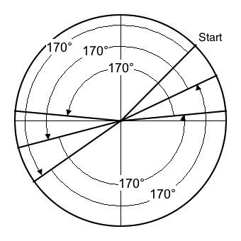
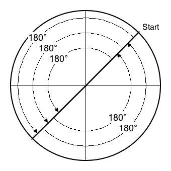
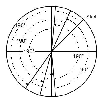
To understand why foldover happens, consider Figure 6-1 through Figure 6-3.
- Figure 6-1 illustrates angular displacements of 170°, which amount to 94% of the Nyquist limit. The sequence of angles is 45°, 215°, 25°, 195°, 5°, and 175°. What results is a signal which alternates between up values and down values, where the up values themselves migrate at a rate of 20° clockwise around the circle. The effect of this migration is to modulate the 94% signal by a second signal which itself alternates 9 up values (since 180°/20° = 9) with 9 down values. So even though we're still short of the Nyquist limit, the generated signal is not as pure as one would prefer.
- Figure 6-2 illustrates angular displacements of 180°, which amount to 100% of the Nyquist limit. The sequence of angles is 45°, 225°, 45°, 225°, 45°, 225°. The up values remained fixed at the starting angle, which in Figure 6-2 produces an intensity of √2/2 = 0.7071. Understand that this intensity depends entirely upon the starting angle. It could be any value ranging from zero to unity. The particular nature of 180° is being its own negative: -180° ≡ 360° - 180° = 180°.
- Figure 6-3 illustrates angular displacements of 190°, which amount to 106% of the Nyquist limit. The sequence of angles is 45°, 235°, 65°, 255°, 85°, 275°. What results is a signal which alternates between up values and down values, where the up values themselves migrate at a rate of 20° counter-clockwise around the circle. This is the same as Figure 6-1 except in the opposite direction, which is unsurprising since 190° ≡ 360° - 170° = -170°. The key point is that Figure 6-1 and Figure 6-3 fill out a unit of time with the same number of up/down cycles, so the resulting waves have the same frequency even if one wave happens to go down when the other goes up.
Video 3 animates an attempt to run a sine-wave generator at frequencies higher than than the Nyquist limit. The video contains two components. The component on the left, labeled Spinner, graphically constructs sine values from particular angles. However, spinner angles are here less of concern than the angular displacements; that is, how much the spinner angle changes from one frame to the next. Small angular displacements generate low frequencies; large angular displacements generate high frequencies. The component on the right, labeled Output, records each newly constructed sine value, then scrolls rightward at a rate of two pixels per frame.
The video lasts 100 seconds overall. The spinner's per-frame angular displacements begin at 45° and widen by equal ratios. 41 seconds into the video, displacements transition upward past the Nyquist threshold of 180°. 50 seconds in, the displacement reaches an upper limit of 252°, at which moment the displacements begin to narrow. 60 seconds in, displacements transition downward though the 180° threshold. Displacements continue to narrow over the remaining duration, returning to the original value of 45°. The audio track which accompanies Video 3 was generated at a rate of 5000 samples per second using an instrument similar to the one shown in Figure 2-2; however, the frequency was controlled by a contour with two exponential segments. The first segment started at 625 Hz. and increased over 50 seconds to 3500 Hz. The second segment started at 3500 Hz. and decreased over 50 seconds to 625 Hz. Why were these frequencies employed? Well 625 Hz. is 1/8 of Hz. 5000 just as 45° is 1/8 of 360°. Likewise 3500 Hz. is 7/10 of Hz. 5000 just as 252° is 7/10 of 360°.
The frame rate for Video 3 has been deliberately ratcheted down to 2.5 frames per second so that you can witness how the direction of angular displacement shifts from counter-clockwise to clockwise during the upward Nyquist transition (41 seconds in). At this point the audio tone stops rising and begins falling. The tone continues falling to the mid-point (50 seconds in). Here the angular displacement shifts from clockwise to counter-clockwise nominal mid-point frequency peak, occuring under foldover conditions, actually comes off as a trough. During the downward Nyquist transition (60 seconds in), the angular displacement shifts from clockwise to counter-clockwise, and the audio tone assumes its expected downard trend.
Video 3: Sine-wave generation by angle-displacements around the unit circle. Displacements increase from 45° initially to 252° mid-way through, then decrease back to 45° at the end. The legend FOLDOVER appears during frames when the angle-displacements exceed 180°. Sample values generated during such frames appear with yellow backgrounds in the signal graph.
The Synthesis Engine
All MUSIC-N sound-synthesis engines work with two input files, an orchestra and a note list
(elsewhere known as a score).
The note list contains statements of various types, the most prominent of which is the
note statement.
Within the Sound engine, each note statement begins with the word “note”, followed by a
sequence of decimal parameters.
Of these, parameters 1-6 have fixed purposes. The present explanation is specifically concerned with parameter #5 (onset time)
and parameter #6 (duration).
Here is how a sound-synthesis engine works in a nutshell.
It first sorts the note statements by order of time, instrument ID, and note ID.
It obtains the end time T from the note list (specifically from an
end statement, of which there must be exactly one), sets the current time
t to 0, and sets note pointer Ni to the first note in the list.
It sets up a currently-playing notes collection, Playing, which is initially empty.
It then loops through the following steps:
- If t ≥ T then exit the loop, we're done!
- Purge all Playing notes with release times (P5+P6) not greater than t.
- Set the play-to time tnext to the next note onset time (P5) or to the minimum release time (P5+P6) of all Playing notes, whichever is smaller.
-
While the onset time (P5) of the Ni equals the t, do the following:
- Initialize the note pointer Ni. This phase of calculation will be examined more closely under the heading Note Initialization.
- Bring Ni into the Playing collection.
- Advance the note pointer Ni to Ni+1.
- Calculate wavefile samples from t up to (but not including) tnext. This phase of calculation will be examined more closely under the heading Audio-Rate Calculations.
- Set the current time t to the play-to time tnext.
Time Granularity
The previous explanation of the synthesis engine described how sample calculations divide into batches. Among other things, the criteria affecting batch sizes includes differences between consecutive note events (start times and end times). Having a cluster of notes which start at nearly the same time could potentially create situations where the engine has to repeatedly cut short batches in order to queue in additional notes.
There is a threshold, however, where nuances of timing become meaningless and where consecutive events are heard to be simultaneous. This threshold is called the “time constant”. It is discussed by Winckel, 1967 pp. 51-55, but seems to have been known back in 1860. The time constant is around 1/18 second, or 55 msec. It represents a number of things, most prominently the transition point between what we perceive as time and what we perceive as frequency. Understand that the time constant is not a precise cutover; for examples:
- The lowest pitch on a pipe organ, 32' C, has a frequency of 16.35 Hz.
- The “steady-state” duration of a liquid consonant can be as short as 30 msec.
The Sound engine granularizes time into 10 msec increments; that is, 100 grains per second.
No matter how many digits a note statement employs after the decimal point,
Sound will round the timing to the nearest 100th of a second.
Dividing the CD standard sample rate of 44,100 by 100 gives 441 samples per channel per grain.
Sound has a default batch length of 1323 samples, which is three time grains.
Audio-Rate Calculation
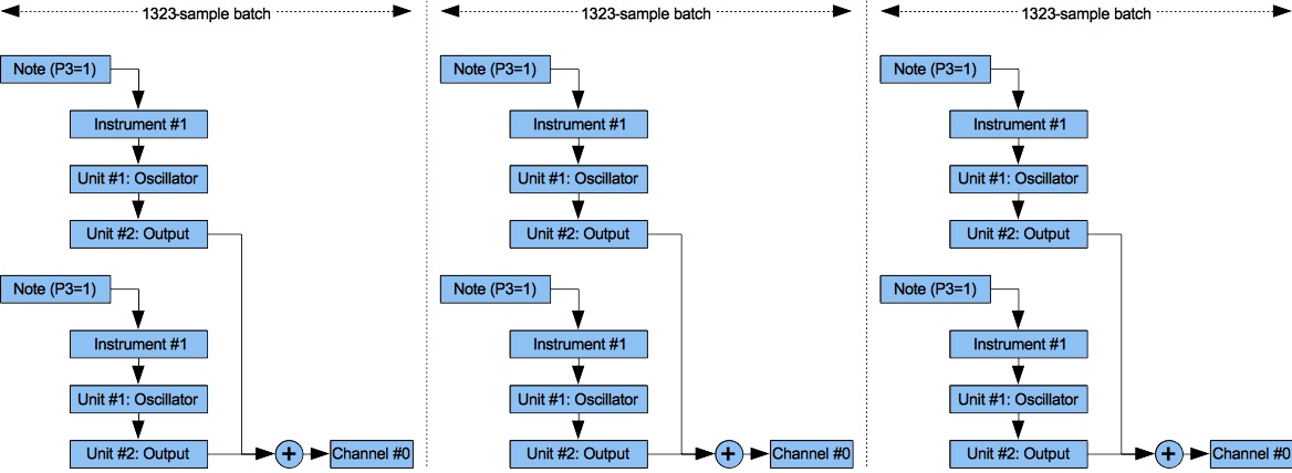
Figure 1: Audio-rate Calculations.
The following text reprises the symbols t, tnext, and tnext, which were defined previously under The Synthesis Engine.
As Figure 1 illustrates, the sound-synthesis engine breaks up the period from t to tnext into batches. The default batch length of 1323 samples (this number is configurable) is enough to process 30 msec of sound at a 44100 Hz. sampling rate. For each batch, the engine iterates through the Playing collection. For each playing note, the engine extracts an instrument number from parameter #3, then sets the corresponding instrument to calculating samples. The instrument in turn delegates calculations to its units. Each type of unit performs calculations in its own peculiar way. The Operation of the Digital Oscillator is instructive.
Once all of the samples in the batch have been mixed together into the output buffers, the output buffers are flushed to file.
The “Simplest” Sound-Synthesis Instrument
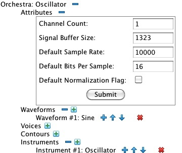
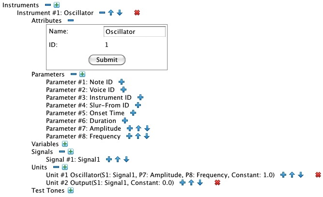
To understand further how sound-synthesis engines work it is necessary to understand instruments, note lists, and in particular how a digital oscillator works. Figure 2-1 and Figure 2-2 depict an orchestra containing what The Technology of Computer Music calls the “simplest instrument”. This specific orchestra will help further explain how samples are calculated, but first a word about orchestra structure generally.
Orchestras contain waveforms and instruments, among other things. You can learn more about waveforms on the Waveform Reference page. Instruments are collections of units linked together through data conduits. Specific unit types are documented on the Unit Reference page. Each unit has a collection of arguments, and each argument references a data conduit. The varieties of data conduit are documented on the Data Conduit Reference page.
|
|
| Figure 2-1: The “simplest orchestra”, viewed through my Orchestra Editor. | Figure 2-2: Expansion of Instrument #1. |
Rather than using the predefined 512-sample sine wave listed as Waveform #1, it will be more instructive to explain things using the 16-sample wave presented in Figure 3 below. This orchestra contains one instrument, as detailed in Figure 2-2. Instrument #1 contains two units: Unit #1 is an Oscillator while Unit #2 is a single-channel Output unit.
While explicit declarations were not required by MUSIC-V, declarations become indispensable in a graphical user interface
where arguments are selected using drop downs.
There are three declarations whose scope is limited to the instrument:
-
The Parameters collection holds declarations of note parameters.
Note parameters are used by the instrument to obtain information from
notestatements in the the note list. Parameters 1-6 are predefined, while the declarations for parameters 7-8 are specific to Instrument #1. - The Variables collection holds declarations for Instrument Variable instances, which are used by instruments to pass single values from unit to unit. Instrument #1 declares no variables.
-
The Signals collection holds declarations for Instrument Signal
instances, which are used by instruments to pass sequences of
and
Signalscollections declare the data elements used to pass information between units of the same instrument. Instrument #1 declares one signal, Signal #1: Signal1.
Here is how the instrument shown in Figure 2-2 operates: The Oscillator unit generates a tone in batches of up to 1323 samples, storing these samples in Signal #1. The tone's zero-to-peak amplitude is controlled by Parameter #7; while tone's frequency is controlled by Parameter #8. The tone's waveform is indicated by the constant value 1, which directs the oscillator to employ Waveform #1.
The Output unit mixes Signal #1 together with what the other notes are contributing to channel #0.
A One-Note Score
orch /Users/charlesames/Scratch/SimplestOrch.xml
set rate 10000
set bits 16
set norm 0
note 1 0 1 0 0.00 0.00 1 32000 440
end 1To make Orchestra #1 produce a sound, we will provide it with the note list presented in Listing 1.
The various statements have the following effects:
-
orch— This statement provides a path to the orchestra definition pictured in Figure 2-1 and Figure 2-2. -
set rate— This statement sets the sampling rate to 10,000 samples per second per channel. Note in Figure 2-1 that the orchestra fixes the number of channels at 1. -
set bits— This statement sets the sample quantization to 16 bits per sample. -
set norm— This statement indicates that the output signal should (1) / should not (0) be normalized so that the largest sample value is 32767. -
note— This statement indicates that the result should contain a note with the following parameters:- The note ID is 1.
- The voice ID is 0 (don't care).
- The note will be generated using instrument #1.
- The slur-from note ID is 0 (No slur-from note).
- The note will start at time 0 (in seconds).
- The note will last for one second.
- The “Amplitude” (as per the definition of parameter #7 in instrument #1) will be 32000.
- The “Frequency” (as per the definition of parameter #8 in instrument #1) will be 440.
-
end— This statement indicates that the output signal will end after 1 second, meaning that the number of samples per channel will be 1 × 10,000 = 10,000.
Note Initialization
MUSIC-V did not do note initialization; however, note initialization became universal in programs of the post-Bell-Labs generation,
including Barry Vercoe's Music360, Vercoe's Music11, and the music program I used at Stanford in 1976.
Vercoe told me that this second generation of sound-synthesis programs were more influenced by MUSIC-IV than MUSIC-V,
and that many MUSIC-IV features were dropped in MUSIC-V in order to permit single instruments to play
simultaneous notes. I am not familiar with MUSIC-IV, but it is possible that note initialization was one of these dropped
features.
The previous heading on the Sound Synthesis Engine placed the note-initialization phase within the overall process of sample calculation; however details of the initialization phase were left for later. I now intend to fulfill this promise. Not having researched what other sound-synthesis engines do during their note-initialization phases, I can only tell you what my Sound engine does. It seems safe to assume that products like Csound and SuperCollider do similar things.
The first thing the engine does in the note-initialization phase is use the instrument id in note parameter #3 to dereference an instrument. The engine next iterates through the instrument's units in unit-ID order, performing one (or neither) of two actions:
- If a unit outputs its results to a variable, then the calculation takes place at this time.
- If the unit needs to retain information from sample to sample, then it must rely on a helper object to store this information. Within the Sound engine, such objects are known as “Cookies”. The structure of a cookie varies with the unit type, but all such cookies cross reference the unit instance (from the instrument) and the note instance (from the note list). If a chain of notes is linked by slurs, then cookies are allocated only once at the beginning of the chain. Whenever a slur-to note initiates, its cookies are retrieved from the corresponding slur-from note.
For an example cookie, refer back to the earlier section, Operation of the Digital Oscillator.
At a bare minimum, each oscillator cookie needs to store what the earlier section called the Phase
variable.
However there are a number of other quantities which do not necessarily need to be recalculated for every sample.
Significant among these quantities is the sampling increment, which only needs
to be recalculated when the input frequency changes.
Voices, Contours, Ramps, and Voice-Level Signals
Four entities, voices, contours, ramps and voice-level signals are implemented by my recent Sound engine but had no equivalents in the sound-synthesis packages I was familiar with during the 1970's. Voices and contours carry through features of my Ashton score-transcription utility, the earliest versions of which were generating note lists in the spring of 1978. This utility organized notes into voices, and it also employed contours to control gradually evolving score-attributes such as tempo and dynamics.
Voices provide a scope for the Sound engine which occupies an intermediate level between the local scope of
note parameters and the global scope of
system variables or of waveforms. In that sense, Sound voices
are analogous to MIDI channels, where you can have many simultaneous notes that all share the same
control information.
However MIDI files transmit single control values at specific moments in time.
By contrast, Sound contours are described by ramp
statements in the note list. Each ramp has a start time, a duration, an origin, and a goal.
Each contour's ramps, placed end-to-end, fill out the entire wavefile duration.
After introducing voices into Sound, it was a logical next step to allow notes from the same voice to pass signals between one another. Voice-level signals enable conditional branching within the sound-synthesis system. For example, suppose you wish to generate a group of tones and noises and then process this specific group of sources through some sort of resonator. You can do that by mixing all the the source outputs into a voice-level signal, then have the resonator pick up this same signal to work its magic.
| © Charles Ames | Page created: 2014-02-20 | Last updated: 2017-08-15 |