Statistical Feedback Demo Instructions

The Demonstrating Applet for statistical feedback allows you to design a scheme of chromas, sounds, chords, and events, then use this scheme to generate a simple composition. Before you try designing schemes of your own, you should check out the five examples I have prepared. Since the applet's file chooser always starts with your home directory, and since you probably don't want to clutter up your home directory with XML files, I recommend that you establish a working folder directly under your home directory. A single working directory will suffice for all the applets on this site.

Version 1.0.8 of the demonstrating applet implements two enhancements relative to the preceding version 1.0.6. The first enhancement is that the SHA-1 64-bit encrypted Java Signing Certificate has been upgraded to 128-bit SHA-2 encryption, as required by the latest browsers. The second enhancement is the establishment of an XML schema document, feedback.xsd. The version 1.0.8 file chooser now verifies that each compliant XML input file has a document element named “example” with a schemaLocation attribute set to “https://charlesames.net/feedback feedback.xsd”. If you wish to understand what is needed to bring a pre-1.0.8 file into compliance, use an online XML validation site such as www.freeformatter.com.

Loading the “Uniform” Example

The first prepared example is defined in the file Feedback-Uniform.xml. Follow the instructions given in here to download this file into a working folder under your home directory.

Initially, the applet should resemble Figure 1.

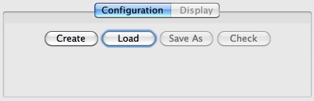
Figure 1: The applet without a file.

To load the file, click on and use the file chooser to locate Feedback-Uniform.xml in its download directory. Once the file is successfully loaded, the applet will display the file path and the topmost component of the configuration scheme. This new display is shown in Figure 2.

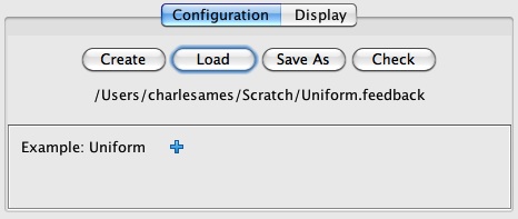
Figure 2: The applet after Feedback-Uniform.xml has been loaded.

Viewing the “Uniform” Configuration

This portion of the instructions explains how to view the components of a feedback example file. If you have loaded one of the five prepared examples and simply wish to experience the demonstration, you may skip ahead to Running the Uniform Example.

We will now tour the graphical editor. Notice that this editor provides no Save or Undo buttons; any changes you make are written directly to the underlying file. That's the bad news. The good news is that if you inadvertently shut down the applet by browsing to another window, you can reload the file you were working on without losing data. You will be called upon to run this example shortly, so don't change any data for the moment.

Document Attributes

The graphical editor employs presents an example file's contents in outline format. Initially the editor displays only Example: Uniform, which is the topmost component of the object hierarchy. To the right of the Example: Uniform is a show-content icon (). Clicking on this icon reveals the child items shown in Figure 3. Notice that the show/expand icon toggles to a hide/collapse icon ().

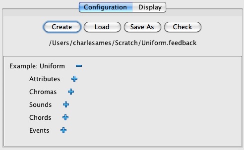
Figure 3: Expanding the Example component reveals five child items.

Expand Attributes by clicking on the item's icon. This action reveals the document-attribute editing panel pictured in Figure 4.

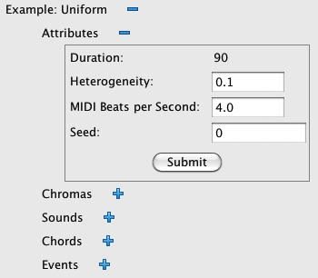
Figure 4: Expanding the Attributes component reveals an attribute-editing panel.

Attribute panels are the exception to the practice of saving changes immediately to file. Within any attribute panel, you make whatever attribute changes you wish and then click on . The editor checks your choices. Only if it agrees with these choices does the editor save the changed attribute values to file.

There are four document attributes:

• Duration — The total length of the composition. This value is calculated as the sum of Event durations. You cannot modify it directly.
• Heterogeneity — This value controls the amount of random leavening introduced into the chord-selection process. More poetically, it measures the bluntness of the knife-edge. When Heterogeneity is small, randomness intervenes only when available options would otherwise affect balance equally. Larger values permit selections to stray from optimal balance; however, the process makes up for such indiscretion in subsequent decisions.
• MIDI Beats per Second — The tempo, expressed in quarter notes per second if the duration unit is treated as a quarter note.
• Seed — Each seed value causes the random number generator to produce a different sequence of random values. If you run an example twice with the same seed — everything else held equal — you'll get the same results.

Take special note of the Hetergeneity and Seed attributes, since you may wish to manipulate these values when you run the example.

Chromas

Continue your tour by hiding () the attributes panel, then expanding () the Chromas collection. The editor should now appear as pictured in Figure 5.

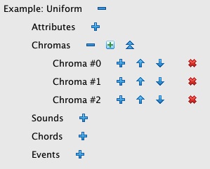
Figure 5: Expanding the Chromas collection reveals list of Chroma items.

Six new control icons are revealed in Figure 5:

• Add new item.
• Resequence items.
• Shift item up.
• Shift item down.
• Push items down.
• Delete item.

We're just looking right now, so don't touch ANY of these. Instead, click on for Chroma #0. Next, click on for both the Attributes and Weight Contour items. The editor should now appear as pictured in Figure 6.

Figure 6: Each Chroma item has an Attributes panel and a Weight Contour.

Figure 6 indicates that Chroma #0 will be displayed using the color BLACK. Chroma #0 will also maintain unit weight through the duration of the piece. Perusing the other two Chroma shows that they also maintain unit weight.

Sounds

Collapse () the Chromas collection and expand () the Sounds collection. Expand Sound #0 and its Attributes panel. The editor should now appear as pictured in Figure 7.

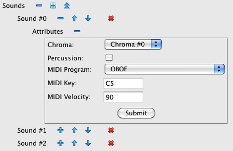
Figure 7: A Sound item with its Attributes panel.

The drop down at the top of the attributes panel in Figure 7 associates Sound #0 with Chroma #0. It also indicates that Sound #0 will be realized aurally using a General Midi oboe playing pitch C5 (an octave above middle C) with MIDI velocity 90 (forte). When the Percussion box is unchecked, the MIDI Key is indicated using a letter name, an accidental (# or !), and an octave number. When the Percussion box is checked, the MIDI Program attribute disappears and the MIDI Key is selected using a drop-down of General MIDI percussion sounds.

Notice you do NOT have control over the MIDI channel. The applet assigns MIDI channels dynamically to MIDI programs, so that two sounds with the same program will be played using the same channel. Since channel #10 is reserved for percussion, no more than 15 different MIDI programs may be selected. However you may define any number of Sounds sharing the same program.

Peruse the other sounds if you wish, then continue the tour by collapsing () the Sounds collection.

Chords

Expand () the Chords collection. This will reveal Chord #0, Chord #1, and Chord #2. Click on for Chord #0 and then click on for the Sounds collection under Chord #0. The editor should now appear as pictured in Figure 8.

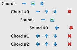
Figure 8: Expanding the Chords collection reveals list of Chord items. Each Chord references one or moure Sound instances.

Figure 8 reveals that Chord #0 simply references Sound #0. If you preruse the other chords, you will discover that Chord #1 references Sound #1 and Chord #2 references Sound #2.

Collapse () the Chords collection.

Events

Continue the tour by expanding () the Events collection. There are 100 Events numbered from 0 to 99. Click on for Event #2 and then click on for the Attributes component under Event #2. The editor should now appear as pictured in Figure 9.

Figure 9: Expanding the Events collection reveals list of Event items. The goal of this demonstration will be to choose a Chord for each Event.

Event components have two attributes, Time and Duration. The Time is derived from the previous event; you cannot modify Time directly. The duration is expressed in quarter notes where the tempo in quarters per second is defined by the document's MIDI Beats per Second attribute. If you peruse the other Events you will discover that all have unit duration.

This completes your tour. Please hide everything but the Example component's attribute panel.

Running the “Uniform” Example

The viewer/editor toured in the previous section is embedded within the first of two tabbed panels named Configuration and Display. The Display panel was initially grayed out (see Figure 1) but came active immediately after Feedback-Uniform.xml was loaded (see Figure 2). However, the Display panel only became active because the applet verified that all the components in Feedback-Uniform.xml were properly defined. Now is the time to click on the tab named Display.

Figure 10: The initial Display panel for Feedback-Uniform.xml.

The Display panel pictured in Figure 10 splits into an upper panel showing the chords and a lower panel showing the sequence of events. The composition will be rendered using a three-line staff; one line each for Chroma #0, Chroma #1, and Chroma #2.

The lower panel has four graphic components.

• The upper row of the lower window presents a Profile showing chroma weights evolve over the duration the composition. Since the weights in Feedback-Uniform.xml are all fixed at unity, the Profile in Figure 10 simply presents three horizontal bars of equal width. The black bar graphs the weight accorded to Chroma #0; the blue bar graphs the weight accorded to Chroma #1; and the cyan (light blue) bar graphs the weight accorded to Chroma #2.
• The lower row of the lower panel starts with a Usage graph. This graph will show, in relative terms, how much of Chroma #0, Chroma #1, and Chroma #2 have been used so far during the selection run. (Such a graph is called a histogram.) Since no Chords have yet been selected, this graph is empty.
• Just right of the Usage graph is a Balance graph showing for each Chroma whether its current usage is balanced (centered hairline) over-balanced (right-extending bar), or under-balanced (left-extending bar). Since no Chords have yet been selected, all three Chroma balances appear as centered hairlines.
• The long staff underneath the Profile depicts the sequence of Event instances. The start of each event is indicated by a vertical line through the staff.

For animation purposes, decisions are broken into three steps. Step 1 calculates for each Chord how the balances will change if the Chord is selected. Step 2 uses the minimax principle to select the chord whose balances stray least around the mid point. Step 3 renders the selected Chord in the event-sequence staff. After Step 3 completes, the process advances to the next Event. The animation completes when a Chord has been selected for every Event. Five buttons control the animation:

	Perform the next step.
	Complete selecting a Chord for the current Event.
	Select Chord instances for every remaining Event at a leisurely rate.
	Select Chord instances for every remaining Event at a rapid rate.
	Interrupt auto-selection.

Click once on . The display panel should resemble Figure 11.

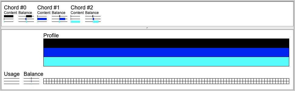
Figure 11: Calculating balances for Event #0.

Each Chord in the upper panel presents a new Balance (per Chord) graph showing how the Balance graph in the lower panel would change if the indicated Chord were to be selected. In general, each Balance-per-Chord graph displays a large positive increment for that particular Chord's Chroma. Notice however that the three graphs are not otherwise similar. In particular, the Balance graph for Chord #0 goes slightly negative for Chroma #1. This is the result of random leavening which is introduced into each balance value. The magnitude of leavening is controlled by the document's Heterogeneity attribute which, as Figure 4 reveals, is smaller than unity (0.1).

Click once again on . The display panel should now appear as in Figure 12.

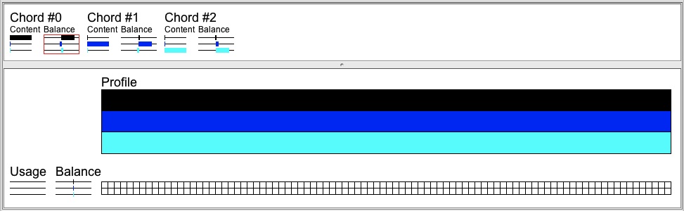
Figure 12: Selecting a Chord for Event #0.

Figure 12 now includes a red border around the Balance graph for Chord #0. Chord #0 is favored because because the balance for Chroma #1 extends farther leftward than any other Chroma balance in any other Chord. Thus the random leavening described above provides the tie-breaker when Chords would otherwise exert influence balance in the same way.

Click for a third time on . The display panel should now appear as in Figure 13.

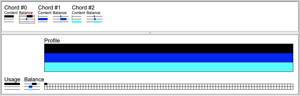
Figure 13: Rendering the Chord for Event #0.

Why does the graph of overall Balance in the lower panel not match the Balance graph for Chord #0? Two reasons:

• The random leavening that skews Chord selection does not figure into the balances of record.
• Each time a Chord is selected, two things happen: First, the balance-of-record for each Chord member is incremented. Second the balances-of-record as a set are normalized so that they sum to zero. The reasons for normalization are complicated. If you want to know more, read my 1990 article, “Statistics and Compositional Balance”

Click on to set loose the remainder of the chord-selection run. When it's finished, the display should resemble Figure 14.

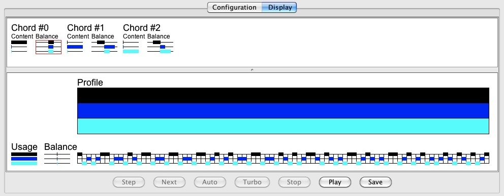
Figure 13: Graphic display for the Feedback-Uniform.xml example after the chord-selection run has completed.

Notice that the Usage graph shows that all three Chroma values have been used in equal amounts. This is what we properly expect when the Chroma weights are uniform.

Notice also that the animation-controlling buttons are all grayed out but that two other buttons have now come active: Click on to hear the a MIDI rendition of the example. Click on to save a MIDI rendition of the example to a file named Uniform.midi.

Building the “Diatonic” Example

This portion of the instructions explains how to create the FeedbackDiatonic.xml example from scratch. This is Example #5 explained on the topic page. You need to read that explanation before you undertake the procedures described here. It will be helpful, but not required, to have read Viewing the Uniform Configuration.

I should warn you up front that building this file will be somewhat tedious. There are 7 Chromas, 11 Chords referencing 22 distinct Sounds, 100 Events and 49 weight-contour segments. Each of these 189 entities requires data entry. I can say that I've done all this myself. Fortunately the 100 Events all have unit durations, so all I had to do there was click on the icon 100 times. (One might be tempted to generate the file using a program, which I myself did for all of the feedback example files).

Make sure you're viewing the Configuration panel. To create a new file, click on . Use the file chooser to locate your working directory and name the file FeedbackDiatonic.xml. If a file with the same name already exists, overwrite it. (You can always re-download the original.) The editor should now resemble Figure 15.

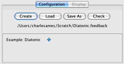
Figure 15: The newly created FeedbackDiatonic.xml example.

Document Attributes

Notice the icon, located just right of the Example component. This is the show/expand icon. Click on it. The editor should now resemble Figure 16.

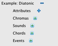
Figure 16: Components of the Example item.

The first thing to do is select document attributes. To reveal the document attributes panel, click on the the show/expand icon () to the right of the Attributes item. The editor should now resemble Figure 17.

Figure 17: The document attributes panel.

The functions of the four document attributes are explained above. Accept all attribute defaults and use the hide/collapse icon () to hide the attributes panel.

Defining Chromas

The next task it to create Chroma components for each of the seven scale degrees. To undertake this task you will need the Chroma table from the example description. Open this link under a separate browser tab.

Locate the Chromas collection and click on the new-item icon (). A New Chroma dialog will appear. Accept the default id (0), and click on . Continue creating Chromas until the display resembles Figure 18: Seven Chromas in all, with id's ranging from 0 to 6. Notice there's no Save option. Each time you create a new Chroma, the change will immediately be recorded in the underlying file.

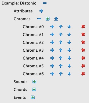
Figure 18: The Chroma collection.

Each Chroma has a color and weight contour. Understand that the scale degrees listed over in the other browser tab are not explicitly coded into the Chroma instances, since Chroma instances do not necessarily stand for scale degrees.

You select a color using the Chroma item's attributes panel. To reveal the attributes panel for Chroma #0, first click on the the show/expand icon () to the right of Chroma #0 item. Two child items will appear: Attributes and Weight Contour. Now click on the to the right of the newly revealed Attributes item.

Figure 19: Attribute panel for Chroma #0.

Change the color to RED; the editor should now resemble Figure 19. Click on . This button tells the editor to check all attributes and, if it likes them, to save them to file. In this particular attribute panel there is only one attribute, the color, and the color has to be valid because it comes from a drop down. However other attribute panels contain values entered using text fields, and those have to be validated.

Continue selecting colors for Chromas using information the Chroma that you earlier opened under a separate browser tab. Once you've selected colors for all seven Chromas, you can close the other browser tab.

Each Chroma defaults to a unit weight holding constant from zero (the start of the example) to infinity. However, the example employs weight contours that change over time. You cannot define weight contours yet because the example has no duration — owing to not yet having any events.

Building the Sounds Collection

To build the Sounds collection you will need the Sounds table from the example description. Open this link under a separate browser tab.

Locate the Sounds collection and click on the new-item icon (). A New Sound dialog will appear. Accept the default id (0), and on . Continue creating Sounds until the collection holds twenty two Sounds in all, with id's ranging from 0 to 21.

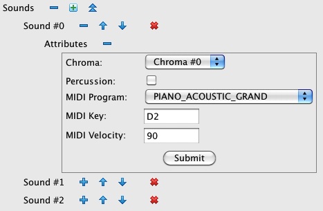
Figure 20: Attribute panel for Sound #0.

Now reveal the attributes panel for Sound #0, which should resemble Figure 20. Perform the following steps:.

• Use the Chroma drop down to select Chroma #0, as indicated for Sound #0 in the other browser tab.
• Leave the Percussion box unchecked.
• Accept the default MIDI Program, ACOUSTIC_GRAND_PIANO.
• Change the MIDI Key to D2, which is the value indicated for Sound #0 in the other browser tab.
• Accept the default MIDI Velocity of 90 (forte).
• Click on

Repeat these steps for each Sound listed in Table 3. Collapse the Sounds collection (). You may also close the other browser tab showing the Sounds table

Building the Chords Collection

The Chord-editing features of the demonstration applet rely entirely on identifiers like “Chord #0” and “Sound #5”. Unfortunately, the Chords table in the example description describes chords in terms of meaningful pitches, not opaque Sound indices. For your convenience, I have converted the pitch-based table into an index-based version, which I present to you here as Table 1.

Chord Index	Sound Index	Sound Index	Sound Index	Sound Index
0	0	13	15	18
1	6	11	13	15
2	6	14	16	20
3	1	7	9	14
4	2	8	11	21
5	3	14	16	18
6	7	11	14	16
7	4	14	15	17
8	8	10	12	14
9	9	11	13	18
10	10	14	15	19

Table 1: Chords for FeedbackDiatonic.xml.

Locate the Chords collection and click on the new-item icon (). A New Chord dialog will appear. Accept the default id (0), and click on . Continue creating Chords until the collection holds eleven Chords in all, with id's ranging from 0 to 10.

Now it's time to fill in the chord content. Expanding Chord #0 reveals the empty Sounds sub-collection pictured in Figure 21.

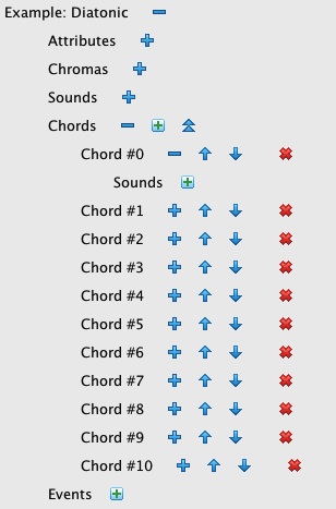
Figure 21: Chord #0 with its Sounds subcollection (initially empty).

Click on the add-item icon (). A Select Sound for Chord #0 dialog will appear. Use the drop-down to select Sound #0, then click on . Use the same steps to add Sounds 13, 15, and 18 to Chord #0. The completed Sounds subcollection is shown in Figure 22.

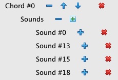
Figure 22: Chord #0 with its Sounds subcollection (completed).

Continue working your way through the rows of Table 4, adding the indicated Sounds to each Chord.

Building the Events Collection

There are two tasks left: (1) defining the sequence of Events; (2) defining a weight contour for each Chroma. The editor will not allow you to extend a weight contour beyond zero until it knows the duration of the example. Therefore building the Events collection is our next task.

We know that the piece lasts 100 quarter notes from the design table in the example description. This time period can be filled in by creating 100 Events, each lasting one quarter note.

Locate the Events collection and click on the new-item icon (). A New Event dialog will appear. Accept the default id (0), and click on . Continue creating Events until the collection contains one hundred Events in all, with id's ranging from 0 to 99. The default duration of any new Event is one quarter note. You can verify this by viewing the attributes panel of whichever event you wish. Figure 23 shows the attributes panel for Event #3.

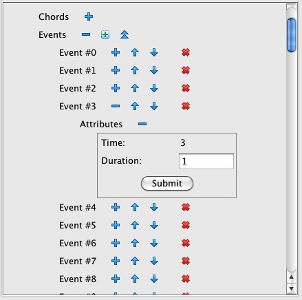
Figure 23: Attributes panel for Event #3.

You can verify that the example now has a total duration of 100 units by reviewing the document attributes panel.

Describing Weight Contours

Now that the editor knows how long the example will last, it will permit you to extend weight contours out beyond time 0. Collapse () everything except for the Chromas collection. Expand () Chromas. Expand Chroma #0, then reveal its weight contour. The editor should now resemble Figure 24.

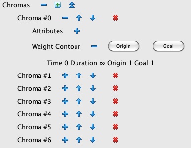
Figure 24: Default weight contour for Chroma #0.

The next series of tables, 2-0 through 2-6, each detail the weight contours for a Chroma as a sequence of segments. Segment properties include start time, duration, origin weight, and goal weight. The first segment start time is always zero; each subsequent statement's start time always equals the end time (start time + duration) of its predecessor. The origin and goal weights are both constrained to the interval from zero to unity (inclusive).

I derived these tables using a short Java program, for which the input was two tables from the example description: Chroma weights for harmonic functions and Harmonic profile for FeedbackDiatonic.xml.

Table 2-0 details the weight contour segments for Chroma #0.

Segment	Time	Duration	Origin	Goal
0	0.0	20.0	1.0	1.0
1	20.0	10.0	1.0	0.5
2	30.0	10.0	0.5	0.5
3	40.0	10.0	0.5	1.0
4	50.0	10.0	1.0	1.0
5	60.0	10.0	0.5	0.5
6	70.0	10.0	0.5	0.0
7	80.0	10.0	0.0	0.0
8	90.0	∞	1.0	1.0

Table 2-0: Weight contour for Chroma #0.

Use the following steps to create this contour:

• Click on . A dialog will appear entitled Weight Origin for Chroma #0. Set the Time to 0 and the Origin to 1, then click on . The display does not change because the weight contours default to static unity, but at least you learned how to create an origin.
• Click on . A dialog will appear entitled Weight Goal for Chroma #0. Set the Time to 20, the Duration to 10, and the Goal to 0.5. Click on .
• Click on again. Set the Time to 40, the Duration to 10, and the Goal to 1.0. Click on .
• Click on . Set the Time to 60 and the Origin to 0.5. Click on .
• Click on . Set the Time to 70, the Duration to 10, and the Goal to 0.0. Click on .
• Click on . Set the Time to 90 and the Origin to 1.0. Click on .

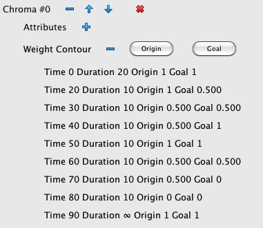
Figure 25: Completed weight contour for Chroma #0.

Figure 25 shows the completed weight contour for Chroma #0. Continue defining weight contours for the remaining Chromas using the information detailed in Table 2-1, Table 2-2, Table 2-3, Table 2-4, Table 2-5 and Table 2-6.

Segment	Time	Duration	Origin	Goal
0	0.0	∞	0.3	0.3

Table 2-1: Weight contour for Chroma #1.

Segment	Time	Duration	Origin	Goal
0	0.0	20.0	0.5	0.5
1	20.0	10.0	0.5	0.3
2	30.0	10.0	0.3	0.3
3	40.0	10.0	0.3	0.5
4	50.0	10.0	0.5	0.5
5	60.0	30.0	0.3	0.3
6	90.0	∞	0.5	0.5

Table 2-2: Weight contour for Chroma #2.

Segment	Time	Duration	Origin	Goal
0	0.0	20.0	0.0	0.0
1	20.0	10.0	0.0	1.0
2	30.0	10.0	1.0	1.0
3	40.0	10.0	1.0	0.0
4	50.0	10.0	0.0	0.0
5	60.0	10.0	1.0	1.0
6	70.0	10.0	1.0	0.5
7	80.0	10.0	0.5	0.5
8	90.0	∞	0.0	0.0

Table 2-3: Weight contour for Chroma #3.

Segment	Time	Duration	Origin	Goal
0	0.0	20.0	0.5	0.5
1	20.0	10.0	0.5	0.3
2	30.0	10.0	0.3	0.3
3	40.0	10.0	0.3	0.5
4	50.0	10.0	0.5	0.5
5	60.0	10.0	0.3	0.3
6	70.0	10.0	0.3	1.0
7	80.0	10.0	1.0	1.0
8	90.0	∞	0.5	0.5

Table 2-4: Weight contour for Chroma #4.

Segment	Time	Duration	Origin	Goal
0	0.0	∞	0.3	0.3

Table 2-5: Weight contour for Chroma #5.

Segment	Time	Duration	Origin	Goal
0	0.0	20.0	0.3	0.3
1	20.0	10.0	0.3	0.0
2	30.0	10.0	0.0	0.0
3	40.0	10.0	0.0	0.3
4	50.0	10.0	0.3	0.3
5	60.0	10.0	0.0	0.0
6	70.0	10.0	0.0	0.5
7	80.0	10.0	0.5	0.5
8	90.0	∞	0.3	0.3

Table 2-6: Weight contour for Chroma #6.

Checking Your Work

If the Display tab is grayed out, click on click on to obtain a list of errors. Such errors usually involve components missing necessary child components. Fix them.

When the Display tab becomes available, activate the Display. Compare the Profile to the Profile graph from the example description. If the two images are not consistent, there must be something wrong with a weight contour. Use the color scheme in Table 1 to identify which Chroma is affected.

If the two images are the same, you are done creating FeedbackDiatonic.xml.